Network Centrality

Measuring Importance and Influence in Networks

SMM638 Network Analytics

What is Centrality?

The Fundamental Question:

Which node is most important in this network?

Two Core Perspectives:

1. Advantageous Position: Who has structural advantages?
   • Access to resources
   • Control over information
   • Influence over others
2. Network Functioning: Who is critical for network operations?
   • Facilitating flows
   • Connecting groups
   • Maintaining coherence

Important

Key Insight: “Importance” depends on context and mechanism

The Centrality Family

Measure	Focus	Question
Degree	Direct connections	Who knows the most people?
Closeness	Reachability	Who can reach everyone quickly?
Betweenness	Brokerage	Who controls information flow?
Eigenvector	Connection quality	Who is connected to important others?
Clustering	Local cohesion	How interconnected is the neighborhood?
PageRank	Prestige	Who receives quality endorsements?

Caution

Each measure captures different aspects of structural importance

Degree Centrality

Definition: Number of direct connections

\[C_D(i) = k_i\]

where \(k_i\) is the number of edges incident to node \(i\)

In Directed Networks:

• In-degree (\(k_i^{in}\)): Incoming connections
• Out-degree (\(k_i^{out}\)): Outgoing connections

Normalized Degree:

\[C_D^{norm}(i) = \frac{k_i}{n-1}\]

where \(n\) is network size

Degree Centrality: Interpretation

Undirected Networks:

• Many friends, contacts, or connections
• High visibility and local influence
• Direct access to information and resources
• Potential for rapid mobilization

Directed Networks:

• High in-degree: Popular, prestigious, sought after
  • Example: Highly cited papers, celebrity Twitter accounts
• High out-degree: Active, gregarious, outgoing
  • Example: Frequent emailers, prolific citers

Warning

Limitations: Ignores indirect connections and network structure beyond immediate neighbors

Degree Centrality: Business Example

R&D Lab Technical Advice Network

High Degree Scientist (sought by 18 colleagues for advice)

• Recognized expert with broad technical knowledge
• Central information hub in the laboratory
• High visibility and influence on research directions
• Risk: Bottleneck for problem-solving, time constraints

Low Degree Scientist (consults with 3 colleagues)

• Focused expertise in specialized area
• May have deep knowledge in niche domain
• Less demand on time for advice-giving
• Opportunity: Develop broader skillset, increase collaboration

Real Pattern: Power-law distribution—few scientists provide most technical advice

Note

Magenta node: High degree (central expert)

Black nodes: ‘7’ is a low degree node example (peripheral)

Closeness Centrality

Definition: Inverse of average distance to all other nodes

\[C_C(i) = \frac{n-1}{\sum_{j \neq i} d(i,j)}\]

where \(d(i,j)\) is the shortest path distance from \(i\) to \(j\)

Alternative (Harmonic Mean):

\[C_C^{harm}(i) = \sum_{j \neq i} \frac{1}{d(i,j)}\]

Intuition: How quickly can node \(i\) reach everyone else?

Note

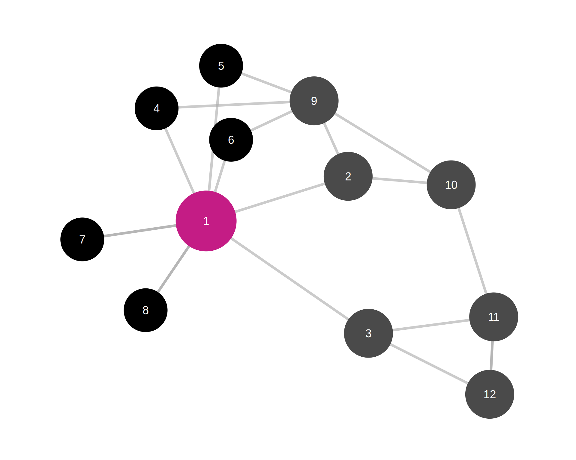
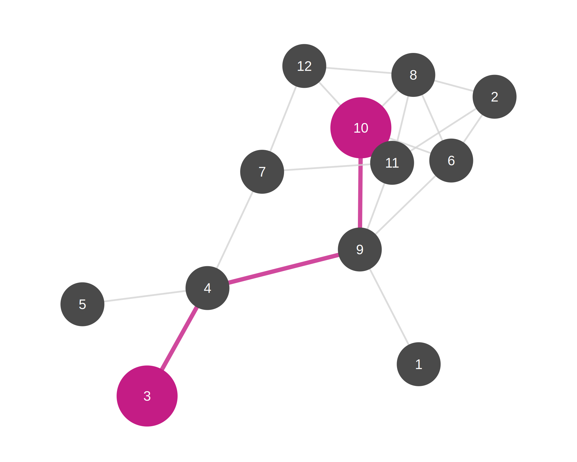
Magenta path: Shortest path between nodes 3 and 10 is through 4 and 9

Closeness considers the shortest path between node \(i\) and all other nodes in the network

Closeness Centrality: Interpretation

What High Closeness Means:

• Can quickly access information from anywhere in network
• Efficient communication with all other nodes
• Potential for rapid dissemination
• Strategic position for time-sensitive activities

Applications:

• Supply chains: Central warehouses minimize delivery times
• Organizations: Managers with high closeness coordinate efficiently
• Epidemic control: High closeness nodes are early infection points
• Innovation: Quick access to diverse information sources

Caution

Limitations: Requires connected network; sensitive to network size; ignores edge weights initially

Closeness Example: Knowledge Networks

Engineering Consulting Firm

High Closeness Engineer (avg distance = 2.1)

• Can quickly reach any expertise in the firm
• Efficient problem-solving through quick consultation
• Ideal for project coordination roles
• Fast knowledge integration

Low Closeness Engineer (avg distance = 4.8)

• Isolated in organizational periphery
• Slower access to firm-wide expertise
• May develop specialized deep knowledge
• Potential: Mentorship to improve integration

Strategic Implication: Closeness predicts coordination effectiveness

Note

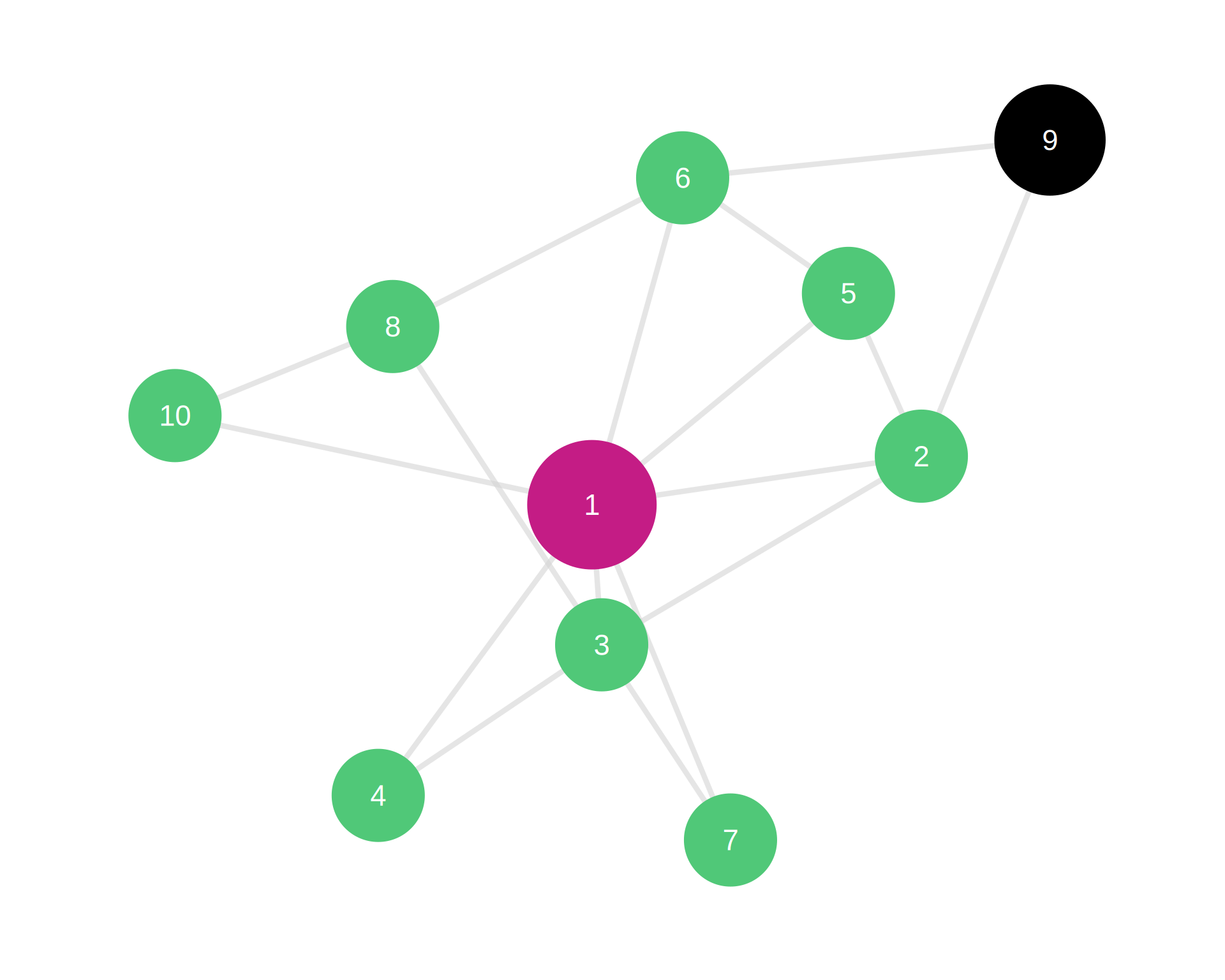
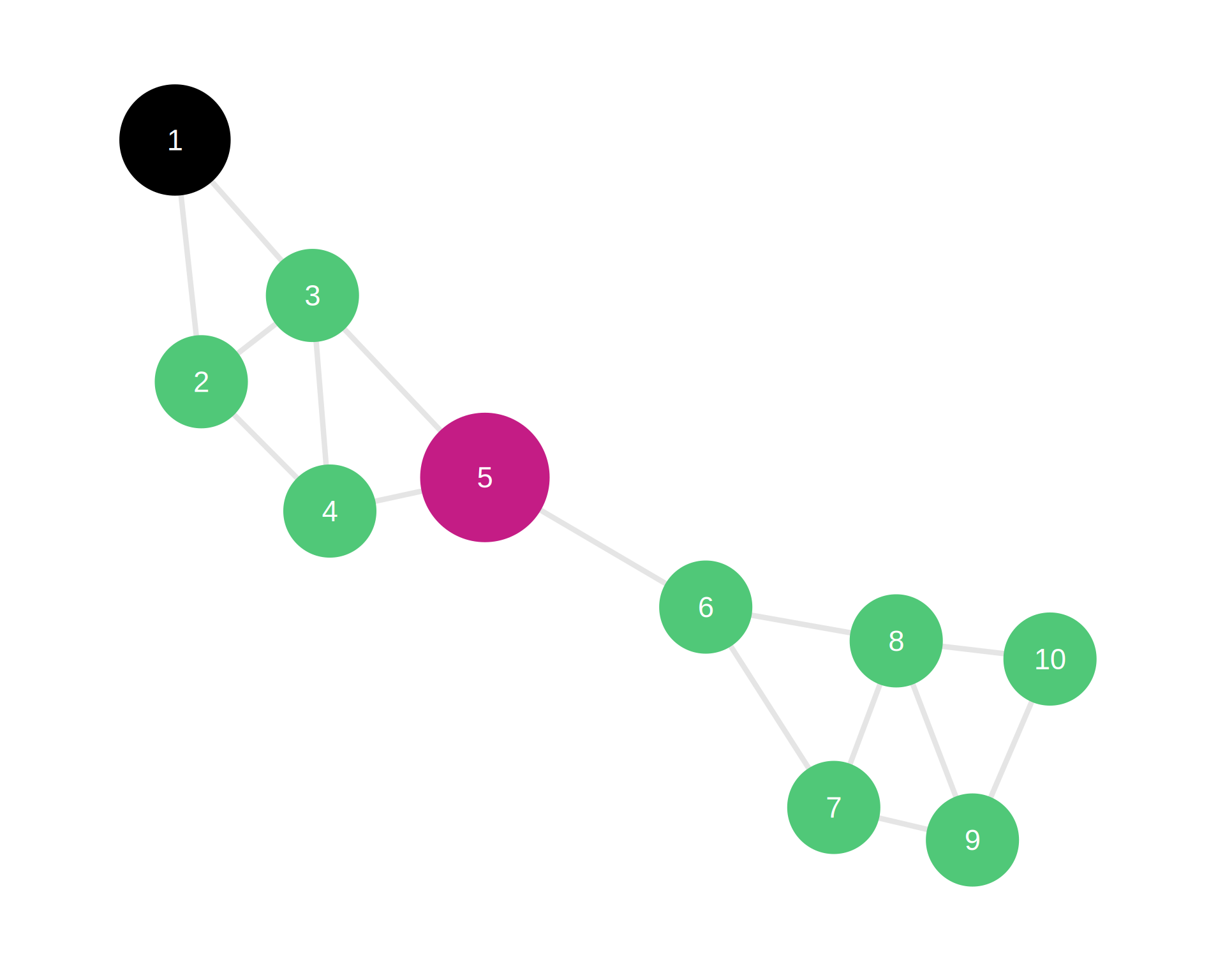
Magenta node: High closeness (central position)

Black node: Low closeness (peripheral position)

Betweenness Centrality

Definition: Proportion of shortest paths passing through a node

\[C_B(i) = \sum_{j<k} \frac{g_{jk}(i)}{g_{jk}}\]

where:

• \(g_{jk}\) = number of shortest paths between \(j\) and \(k\)
• \(g_{jk}(i)\) = number of those paths passing through \(i\)

Normalized:

\[C_B^{norm}(i) = \frac{2 \cdot C_B(i)}{(n-1)(n-2)}\]

Betweenness: The Broker Position

What High Betweenness Means:

• Controls information flow between others
• Broker between different groups or communities
• Can delay, distort, or facilitate communication
• Structural hole position (Burt’s theory)

Strategic Value:

• Information arbitrage: Access to diverse information
• Gatekeeping power: Control what information passes
• Innovation potential: Recombination of ideas from different groups
• Political capital: Both sides need the broker

Important

Risk: Bottleneck position—removal disrupts network flow

Betweenness Example: Innovation Networks

Pharmaceutical R&D Network

High Betweenness Scientist (bridges Chemistry & Biology labs)

• Unique position connecting two specialized domains
• Controls knowledge transfer between groups
• First to see combination opportunities
• Career advantage: Valuable to both groups
• Organizational value: Enables cross-disciplinary projects

Low Betweenness Scientist (within dense cluster)

• Embedded in single community
• Many redundant paths don’t pass through them
• Deep specialization possible
• Innovation: Incremental improvements

Finding: High betweenness predicts cross-disciplinary breakthroughs

Note

Magenta node: High betweenness (broker position)

Black node: Low betweenness (embedded in group)

Eigenvector Centrality

Definition: Centrality proportional to sum of neighbors’ centralities

\[x_i = \kappa^{-1} \sum_{j} A_{ij} x_j\]

In matrix form: \(\mathbf{Ax} = \kappa \mathbf{x}\)

where \(\mathbf{x}\) is the leading eigenvector of adjacency matrix \(\mathbf{A}\)

Key Insight: You’re important if you’re connected to important people

Recursive Logic: Node centrality depends on neighbors’ centrality, which depends on their neighbors’ centrality, etc.

Eigenvector Centrality: Quality vs. Quantity

Degree vs. Eigenvector:

• Degree: Counts all connections equally (1 point per neighbor)
• Eigenvector: Weights neighbors by their importance

Example Scenarios:

Scenario A: High Degree, Low Eigenvector

• 50 connections to peripheral nodes
• “Popular among the unpopular”
• Volume without prestige

Scenario B: Low Degree, High Eigenvector

• 3 connections to highly central nodes
• “Connected to the elite”
• Quality over quantity

Note

Classic Example: Craig Robinson (former Oregon State basketball coach) has high eigenvector centrality because he’s President Obama’s brother-in-law

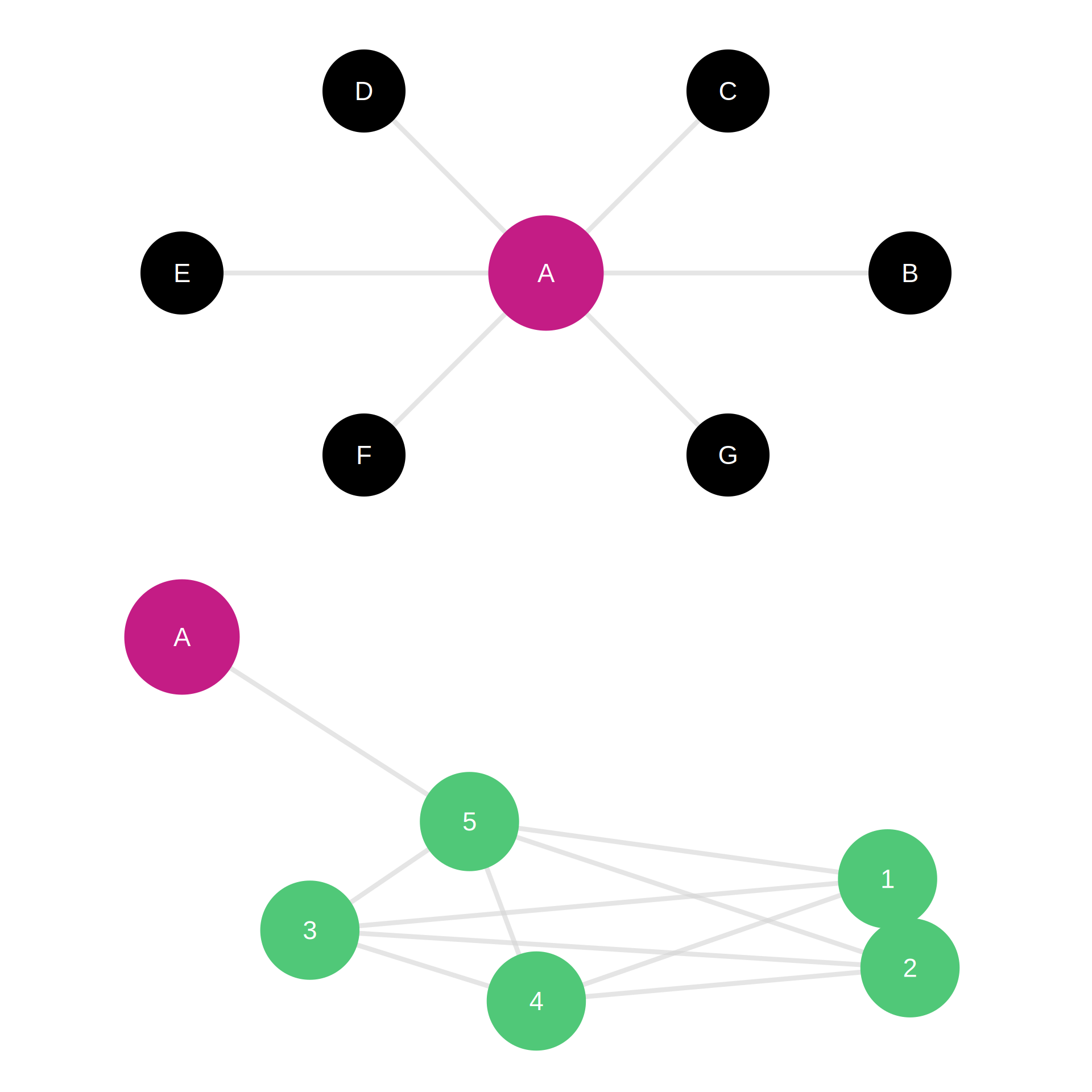
Note

Top network (Scenario A): Node A (magenta) has high degree (6 connections) but low eigenvector centrality (connected to peripheral nodes shown in black)

Bottom network (Scenario B): Node A (magenta) has low degree (1 connection) but high eigenvector centrality (connected to highly central cluster shown in emerald)

Eigenvector Example: Venture Capital

Startup Funding Network

High Eigenvector VC Firm

• Invests alongside other prestigious VCs
• Connected to successful entrepreneurs
• Signals quality to market
• Attracts top deal flow
• Co-investment opportunities with elite partners

Low Eigenvector VC Firm

• Invests with less established partners
• May take more risks on unproven teams
• Less signaling value
• Opportunity: First-mover on emerging trends

Empirical Finding: High eigenvector centrality VCs achieve higher returns (network effects in syndication)

Clustering Coefficient

Definition: Proportion of neighbors that are also connected

\[C_{clust}(i) = \frac{2e_i}{k_i(k_i-1)}\]

where:

• \(k_i\) = degree of node \(i\)
• \(e_i\) = number of edges between neighbors of \(i\)

Interpretation: How interconnected is node \(i\)’s neighborhood?

Range: 0 (no neighbors connected) to 1 (all neighbors connected)

Key Insight:

• Closed triad: Node’s neighbors are connected → High clustering
• Open triad: Node’s neighbors are not connected → Low clustering

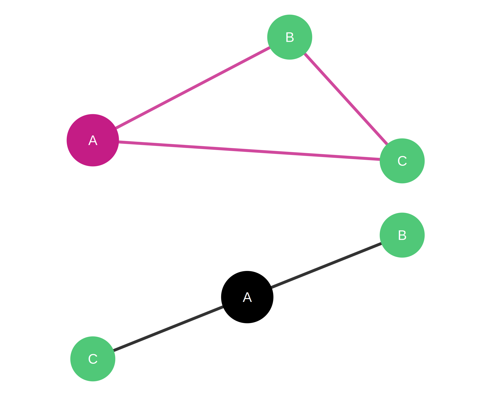
Note

Top network (Closed triad): Node A (magenta) has clustering coefficient = 1.0. Both neighbors B and C (emerald) are connected to each other.

Bottom network (Open triad): Node A (black) has clustering coefficient = 0.0. Neighbors B and C (emerald) are not connected.

Clustering Coefficient: Embeddedness

What High Clustering Means:

• Node is part of a dense, cohesive group
• High social capital and trust
• Information redundancy (everyone knows everyone)
• Strong group norms and social control
• Closure benefits (Coleman’s theory)

What Low Clustering Means:

• Node bridges disconnected groups
• Access to diverse, non-redundant information
• Weak tie advantages (Granovetter’s theory)
• Brokerage opportunities
• Less embedded, more autonomous

Trade-off: Closure (trust, coordination) vs. Brokerage (novelty, diversity)

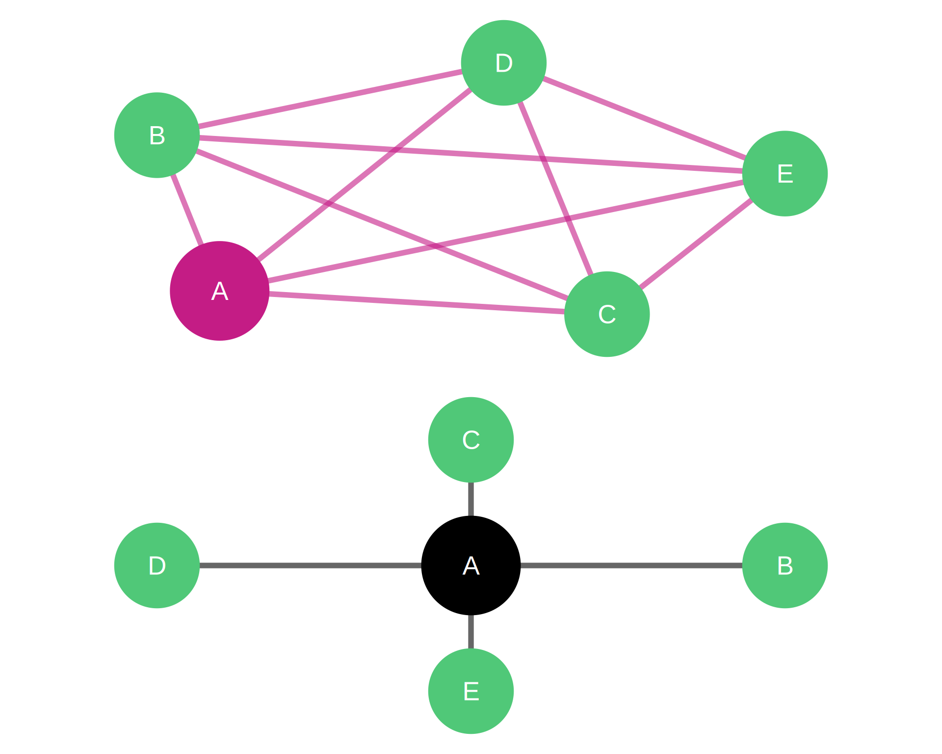
Note

Top network (High Clustering): Node A (magenta) is embedded in a dense, cohesive group where neighbors B, C, D, E (emerald) are highly interconnected. Closure benefits.

Bottom network (Low Clustering): Node A (black) bridges disconnected groups. Neighbors B, C, D, E (emerald) are not connected to each other. Brokerage opportunities.

Clustering Example: Scientific Collaboration

Academic Research Networks

High Clustering Professor (clustering = 0.85)

• Collaborators know and work with each other
• Cohesive research group or lab
• Efficient coordination and shared understanding
• Strong collective identity
• Publication pattern: Multiple coauthors from same institution
• Risk: Echo chamber, less novelty

Low Clustering Professor (clustering = 0.15)

• Collaborators don’t overlap
• Bridges multiple research communities
• Access to diverse methods and ideas
• Publication pattern: Different coauthors for different papers
• Potential: Interdisciplinary breakthroughs

PageRank

Definition: Prestige based on quality of incoming links

\[PR(i) = \frac{1-d}{n} + d \sum_{j \in M(i)} \frac{PR(j)}{L(j)}\]

where:

• \(d\) = damping factor (typically 0.85)
• \(M(i)\) = nodes linking to \(i\)
• \(L(j)\) = number of outgoing links from \(j\)

Key Innovation: Endorsement from important nodes counts more

Origin: Google’s original ranking algorithm for web pages

PageRank: Beyond Google

The “Random Surfer” Model:

• Imagine surfer clicking links randomly
• Sometimes (15%) jumps to random page
• PageRank = probability of finding surfer at each page
• High PageRank = frequently visited in random walks

Advantages over Eigenvector:

• Handles directed networks better
• Deals with dangling nodes (no outlinks)
• Dampening factor prevents pathological cases
• More robust in practice

PageRank Example: Twitter Influence

Social Media Network Analysis

High PageRank Account

• Followed by other influential accounts
• Endorsements carry weight
• Information cascades originate here
• Real influence beyond follower count

Comparison:

• Account A: 100K followers, mostly inactive accounts (low PageRank)
• Account B: 10K followers, including journalists and celebrities (high PageRank)

Marketing Insight: PageRank identifies true influencers, not just popular accounts

Application: Influencer identification, opinion leader detection, cascade prediction

Comparing Centrality Measures

Correlations and Divergences:

Often Correlated:

• Degree and Eigenvector (well-connected tends to connect to well-connected)
• Closeness and Degree in many networks
• Betweenness and low clustering (brokers bridge groups)

Can Diverge:

• High degree but low betweenness (dense cluster member)
• High betweenness but low degree (critical bridge with few ties)
• High eigenvector but low degree (connected to few important others)

Recommendation: Calculate multiple measures; triangulate interpretations

When to Use Which Measure

Selection Guide:

Use Case	Recommended Measure	Why
Identify popular individuals	Degree (in)	Direct connections matter
Find information hubs	Closeness	Quick access to all
Locate brokers	Betweenness	Control over flows
Detect prestigious actors	Eigenvector or PageRank	Quality of connections
Assess group cohesion	Clustering	Local density
Rank web pages	PageRank	Link endorsement
Predict influence spread	Eigenvector + Betweenness	Reach and position

Centralization vs. Centrality

Important Distinction:

Centrality (Node-level):

• Individual scores for each node
• Distribution across network
• Who is most central?

Centralization (Network-level):

• Overall concentration of centrality
• Single score for entire network
• How centralized is the structure?

Formula (Freeman):

\[C = \frac{\sum_i [C_{max} - C_i]}{max\sum [C_{max} - C_i]}\]

Range: 0 (all equal) to 1 (perfect star)

Applications Across Domains

Marketing:

• Identify influencers (high eigenvector/PageRank)
• Target opinion leaders (high betweenness)
• Viral marketing strategies (high closeness)

Operations:

• Supply chain resilience (betweenness analysis)
• Knowledge management (closeness optimization)
• Communication efficiency (clustering + closeness)

HR & Organizational Design:

• Talent identification (eigenvector centrality)
• Team composition (balance clustering/brokerage)
• Succession planning (dependency on high betweenness)

Limitations and Caveats

Methodological Challenges:

1. Boundary specification: Who/what to include?
2. Missing data: Incomplete networks bias results
3. Temporal dynamics: Networks change over time
4. Multiple relations: Which ties matter?
5. Context dependence: Same position, different meanings
6. Correlation ≠ causation: Structure reflects and shapes behavior

Best Practices:

• Use multiple measures
• Consider substantive interpretation
• Validate with qualitative data
• Test robustness to specifications

Key Takeaways

Important

Core Concepts:

1. Centrality measures importance, but importance is multidimensional
2. Different measures capture different mechanisms and advantages
3. Context matters: Same structure, different meanings
4. Centrality distributions reveal inequality and vulnerability
5. Compare multiple measures for comprehensive understanding

Note

Practical Wisdom:

• No single “best” centrality measure
• Match measure to substantive question
• Consider computational constraints
• Interpret in context of research question