Dyads, Triads, and Network Dynamics

SMM638 Network Analytics

Week 4 Overview

Key Questions:

Why do networks look the way they look?
What processes generate network structures?
How can we test for and model these processes?

Topics:

Taxonomy of network formation mechanisms
Dyadic and triadic processes
Statistical tests for network effects
Exponential Random Graph Models (ERGMs)
Network dynamics

Why Do Networks Look the Way They Look?

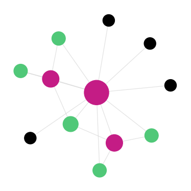
Networks are not random - they exhibit consistent structural patterns:

Clustering: Friends of friends tend to be friends
Degree heterogeneity: Some nodes have many connections, others few
Homophily: Similar nodes connect more often
Small world: Short path lengths despite local clustering

Central Question: What social, biological, or physical processes create these patterns?

Typical network: hubs, clusters, paths

The Formation Question

Two complementary perspectives:

Structural mechanisms: Network topology drives new connections
- Example: Triadic closure creates clusters
Attribute-based mechanisms: Node characteristics drive connections
- Example: Homophily - similarity breeds connection

Challenge: Disentangling these effects requires sophisticated statistical models

Taxonomy of Network Effects

Major categories of network formation processes:

Category	Description	Example
Dyadic	Two-node processes	Homophily, reciprocity
Triadic	Three-node processes	Transitivity, balance
Higher-order	Four+ node processes	K-cores, cliques
Node-level	Individual preferences	Preferential attachment
Exogenous	External factors	Geography, institutions

Dyadic Processes: Definition

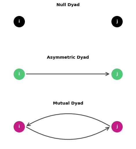
Dyadic processes operate on pairs of nodes (dyads)

A dyad can be in three states:

Null: No connection (i → j and j → i both absent)
Asymmetric: One-way connection (i → j OR j → i)
Mutual: Two-way connection (i → j AND j → i)

Dyadic processes explain why specific pairs of nodes connect

Dyadic Process: Reciprocity

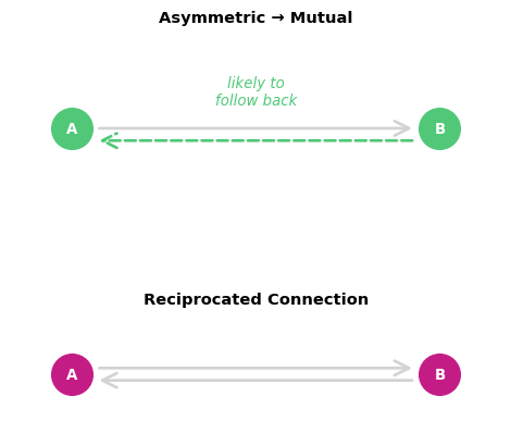
Definition: The tendency for directed edges to be reciprocated

Mechanism: If i → j exists, j → i becomes more likely

Examples:

Social media: You follow back those who follow you
Collaboration: Co-authorship often becomes bidirectional
Trade: Countries with import relationships develop export relationships

Statistical signature: Higher proportion of mutual dyads than expected by chance

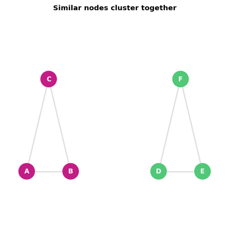
Dyadic Process: Homophily

Definition: “Similarity breeds connection” - nodes with similar attributes connect more

Types:

Demographic: Age, gender, ethnicity
Behavioral: Interests, activities
Status: Education, occupation

Formula: \(Pr(e_{ij} = 1 | phi(A_{i}, A_{j}))\)

where \(\phi\) is a similarity or distance function.

Empirical Evidence:

Wikipedia editors (Crandall et al., 2008): Editors with similar editing patterns more likely to communicate
University email network (Kossinets & Watts, 2006): Students taking same classes form connections at higher rates

Dyadic Process: Homophily vs Selection

Critical distinction:

Selection (homophily): Similar people connect
Influence: Connected people become similar

Problem: Observational data shows correlation, not causation!

Empirical example - Wikipedia editors (Crandall et al., 2008):

Tracked similarity over time relative to first communication
Before contact: Rapid increase in similarity (selection)
After contact: Continued slower increase (influence)
Both processes operate simultaneously!

Solutions:

Longitudinal data tracking changes over time
Statistical models that separate effects (e.g., SAOMs)
Natural experiments

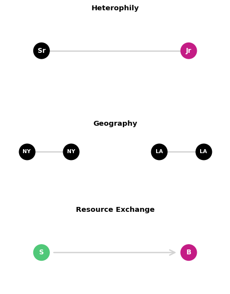
Other Dyadic Processes

Heterophily: Attraction to difference (opposite of homophily)

Example: Dating networks, mentor-mentee relationships

Distance/Geography: Physical proximity increases connection probability

Example: Friendship networks, communication patterns

Status homophily: Nodes connect within same status level

Example: Corporate networks, academic citations

Resource exchange: Complementary needs drive connections

Example: Economic networks, mutualistic relationships

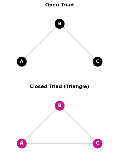
Triadic Processes: Definition

Triadic processes involve three nodes forming triangles

Key configurations:

Open triad: A-B, B-C exist but A-C absent
Closed triad (triangle): A-B, B-C, and A-C all exist

Core insight: The presence of two edges affects the probability of the third

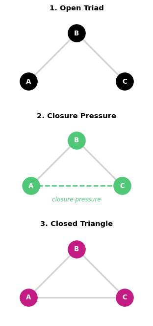
Triadic Process: Transitivity

Definition: “Friends of friends become friends”

Mechanism: If A→B and B→C, then A→C becomes more likely

Also called: Triadic closure, clustering

Examples:

Social networks: Introduced through mutual friends
Academic collaboration: Co-authors of co-authors collaborate
Protein networks: Proteins interacting with same partner interact

Measurement: Clustering coefficient, transitivity ratio

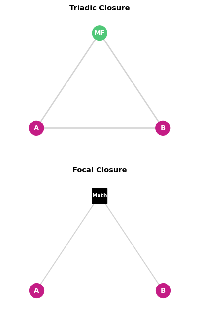
Empirical Evidence: Triadic & Focal Closure

Kossinets & Watts (2006)³: Email network at large US university

Data: ~22,000 students over one year

Key findings:

Triadic closure (shared friends):

Probability increases roughly linearly with common friends
Strong effect: 2 common friends > 2× effect of 1 friend

Focal closure (shared activities/classes):

First shared class has similar effect to one friend
Diminishing returns for additional classes
Curve levels off (different from triadic closure)

Implication: Both structural and contextual effects matter!

³ Kossinets, G., & Watts, D. J. (2006). Empirical analysis of an evolving social network. science, 311(5757), 88-90.

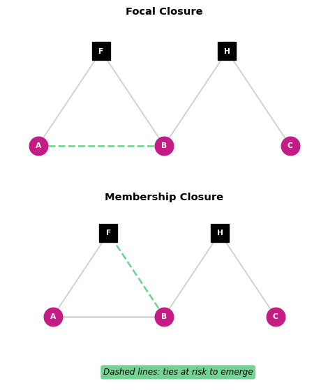
Focal vs Membership Closure: Key Distinction

Focal Closure (Easley & Kleinberg, 2010)²:

People meet through shared activities/contexts (foci)
Examples: Classes, workplaces, clubs, events
Mechanism: Physical proximity + repeated interaction
Pattern: Bipartite structure (people ↔︎ activities)

Membership Closure:

People connect through shared group memberships
Examples: Organizations, committees, teams
Mechanism: Formal affiliation creates opportunities
Pattern: Overlapping group boundaries

Key insight: Context matters as much as network structure!

² Easley, D., & Kleinberg, J. (2010). Networks, crowds, and markets: Reasoning about a highly connected world (Vol. 1). Cambridge: Cambridge university press.

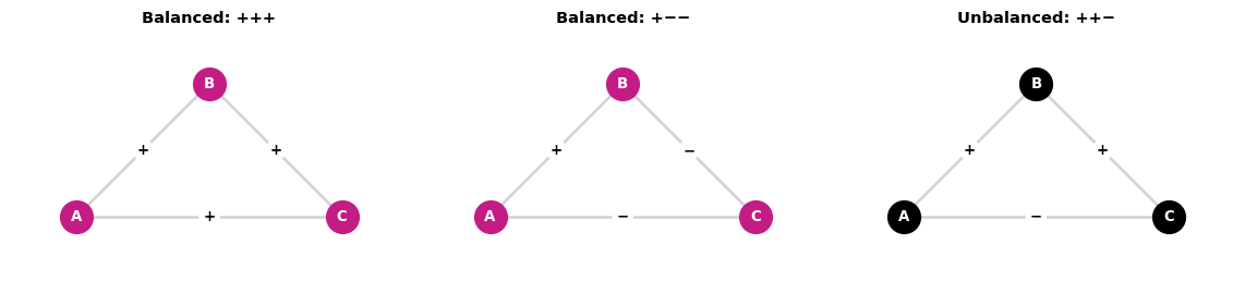
Triadic Process: Balance Theory

Structural balance (Heider, 1946): Cognitive consistency in signed networks

Balanced triangles (all relationships consistent):

+++: Three mutual friends (stable)
+–: Two enemies share a common enemy (stable)

Unbalanced triangles (tension):

++-: Friend of friend is enemy (unstable)
—: Three mutual enemies (unstable)

Prediction: Networks evolve toward balanced states

Triadic Configurations in Directed Networks

16 possible triadic configurations (triads census)¹:

Key patterns:

003: Empty (no edges)
012: One edge only
102: Two edges, no transitivity
030T: Transitive triple
300: Complete triangle

Different processes favor different configurations

Each tells us something about network formation mechanisms!

¹ Vladimir Batagelj and Andrej Mrvar, A subquadratic triad census algorithm for large sparse networks with small maximum degree, University of Ljubljana, http://vlado.fmf.uni-lj.si/pub/networks/doc/triads/triads.pdf

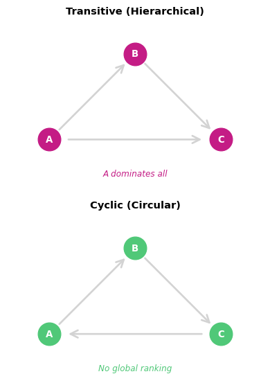
Triadic Process: Cyclicity vs Transitivity

Transitivity: A→B→C implies A→C (hierarchical)

Creates hierarchies, rankings
Example: Citation networks, food webs

Cyclicity: A→B→C implies C→A (circular)

Creates exchange cycles
Example: Rock-paper-scissors, circular status

Distinction matters for understanding network function!

Statistical Tests for Network Effects

Challenge: Network data violates independence assumptions

Classical approach fails: Standard statistical tests assume independent observations

Solutions:

Permutation tests: Randomize while preserving structure
Conditional Uniform Graph (CUG) tests: Compare to random graphs
Quadratic Assignment Procedure (QAP): Correlation with permutation

Permutation Tests for Networks

Logic:

Calculate observed statistic (e.g., clustering)
Generate random networks preserving certain properties
Calculate statistic on random networks
Compare: Is observed value extreme?

Key decision: What to preserve when randomizing?

Node degrees?
Number of edges?
Dyad distributions?

Graph Uniform Test

In network analyses, permutation tests are often called Graph Uniform Tests.

Purpose: Test whether an observed network differs significantly from random networks

Fundamental Aspects:

Null Hypothesis: Observed network is drawn from a uniform distribution of graphs
Test Statistic: Any network property (density, clustering, centralization, etc.)
Procedure:
1. Calculate test statistic on observed network
2. Generate many random networks with same size and density
3. Calculate test statistic for each random network
4. Compare observed statistic to distribution of random statistics

Interpretation: - p < 0.05: Network structure differs significantly from random - p ≥ 0.05: Cannot reject that network is random

Applications: Detect non-random patterns in social networks, communication networks, biological networks

QAP Regression

Quadratic Assignment Procedure: Test relationship between network matrices

Use case: Does network Y depend on network X?

Example: Does friendship (Y) depend on geographic proximity (X)?

Procedure:

Regress Y on X, get coefficient β
Permute rows/columns of Y simultaneously
Repeat regression, get β*
Repeat 1000+ times
P-value: proportion where |β*| > |β|

Advantage: Accounts for network dependencies

Exponential Random Graph Models (ERGMs)

Core idea: Model probability of observing a network as function of its features

Form: \[P(Y = y) = \frac{1}{\kappa} \exp\left(\sum_k \theta_k s_k(y)\right)\]

Where:

\(Y\): Random network
\(s_k(y)\): Network statistics (edges, triangles, etc.)
\(\theta_k\): Parameters (effects to estimate)
\(\kappa\): Normalizing constant

ERGM: Intuition

Think of it as logistic regression for networks

Instead of: P(person votes yes) = f(age, income, …)

We have: P(network has this structure) = f(edges, triangles, homophily, …)

Key insight: Model entire network as outcome, not individual ties

Advantages:

Tests multiple mechanisms simultaneously
Controls for confounding effects
Provides effect sizes, not just significance

Common ERGM Terms

Term	Effect	Interpretation
`edges`	Density	Overall connection probability
`mutual`	Reciprocity	Tendency for reciprocation
`triangle`	Transitivity	Tendency for closure
`nodematch("attr")`	Homophily	Same-attribute connection
`nodecov("attr")`	Attribute effect	Node attribute influence
`gwesp`	Shared partners	Weighted transitivity

Model specification: Choose terms based on theory!

ERGM: Interpretation

Positive coefficient (θ > 0): Configuration is more likely than chance

Negative coefficient (θ < 0): Configuration is less likely than chance

Example interpretation:

edges: -2.5    (low baseline density)
mutual: 1.8    (strong reciprocity)
triangle: 0.4  (moderate transitivity)
nodematch("gender"): 0.6  (gender homophily)

Reading: Controlling for density, reciprocity, and triangles, same-gender ties are more likely

ERGM: Challenges

Degeneracy problem: Some specifications lead to extreme networks

All edges or no edges
Complete clustering or no clustering

Computational challenge: Calculating κ is often intractable

Solutions:

Use geometrically-weighted terms (GWESP, GWDSP)
Markov Chain Monte Carlo (MCMC) estimation
Careful model specification and testing

Network Dynamics Models

So far: Models of static networks (single time point)

Reality: Networks evolve over time

Dynamic approaches:

Temporal ERGMs: ERGMs on network changes
Stochastic Actor-Oriented Models (SAOMs): Actor-driven change
Relational Event Models (REMs): Continuous-time interactions

Stochastic Actor-Oriented Models

Key assumption: Actors make rational decisions about ties

Process:

Actors get random opportunities to change ties
They evaluate potential changes via utility function
They choose change that maximizes utility

Utility function includes:

Structural preferences (transitivity, reciprocity)
Attribute preferences (homophily)
Costs and benefits

Software: RSiena package in R

Advantage: Separates selection from influence effects!

```

Comparing Modeling Approaches

Approach	Time	Question	Strength
ERGM	Static	What structure?	Multiple mechanisms
SAOM	Panel	How does it change?	Selection vs influence
REM	Continuous	When do events occur?	Precise timing
TERGM	Discrete steps	What changes?	Network evolution

Choice depends on:

Data structure (cross-sectional vs longitudinal)
Research question (structure vs process)
Computational resources

Summary: Key Takeaways

Network structure emerges from systematic processes, not randomness
Dyadic processes (reciprocity, homophily) explain pairwise connections
Triadic processes (transitivity, balance) explain local clustering
Statistical tests must account for network dependencies (permutation, QAP)
ERGMs model network probability as function of multiple mechanisms
Dynamic models capture how networks evolve over time

Next steps: Applying these models to real data!