Communities, Roles, and Positions in Networks

SMM638 Network Analytics

Part I: Network Communities

Overview of Weeks 1–5

Important

What we have learned:

  • Network Representation: Nodes (actors), edges (relationships), and the “physics” of connectivity.
  • Node Positioning: Centrality metrics (Degree, Betweenness, Eigenvector) to identify key players.
  • Formation Mechanisms: Why links form (Homophily, Triadic Closure, Preferential Attachment).

Caution

What we will learn (Weeks 7 & 8):

  • Macro-Structure (Communities):
    • Detecting cohesive subgroups (cliques, clusters).
    • Business Use: Market segmentation, fraud rings, organizational silos.
  • Meso-Structure (Roles & Positions):
    • Identifying actors with similar functions (even if unconnected).
    • Business Use: Talent management, supply chain redundancy, competitive analysis.
  • Strategic Implications:
    • How structure dictates performance, innovation, and resilience.

Why Do Networks Are More Than the Sum of Their Parts?

Sociologist Émile Durkheim proposed two forms of social integration that map perfectly onto network analysis, and explain why networks are more than the sum of their parts:

1. Mechanical Solidarity (Cohesion)

  • Integration through similarity and direct interaction.
  • “We are connected because we are the same.”
  • Network Concept: Communities (Clusters, Cliques).

2. Organic Solidarity (Equivalence)

  • Integration through interdependence and specialized roles.
  • “We are connected because we need each other’s different functions.”
  • Network Concept: Positions (Roles, Blockmodels).

Key Insight: A network can be analyzed through cohesion (who hangs out with whom) or equivalence (who does the same job).

Example: Academic Department

Code
library(igraph)

# 1. Construct the Network (Edges based on Community Cohesion)
edges <- data.frame(
  from = c("Prof_A", "Prof_A", "PhD_1",   # ML Group
           "Prof_B", "Prof_B", "PhD_3"),  # Theory Group
  to   = c("PhD_1",  "PhD_2",  "PhD_2",
           "PhD_3",  "PhD_4",  "PhD_4")
)
g <- graph_from_data_frame(edges, directed = FALSE)

# 2. Define Attributes (Data from Example)
# Communities (Color)
V(g)$color <- ifelse(V(g)$name %in% c("Prof_A", "PhD_1", "PhD_2"), 
                     "#E41A1C", "#377EB8") # Red for ML, Blue for Theory

# Positions (Shape)
# Profs are Squares, Students are Circles
V(g)$shape <- ifelse(V(g)$name %in% c("Prof_A", "Prof_B"), 
                     "square", "circle")

# 3. Visualize
par(mar=c(1,1,1,1))
plot(g, layout = layout_nicely(g),
     vertex.label.color = "white", vertex.label.font = 2,
     vertex.size = 30, edge.width = 2,
     main = "Communities (Color) vs. Positions (Shape)")

legend("bottomleft", legend = c("ML", "History"), 
       col = c("#E41A1C", "#377EB8"), pch = 19, bty = "n", title = "Community")
legend("bottomright", legend = c("Senior", "Junior"), 
       col = "black", pch = c(15, 16), bty = "n", title = "Position")

A junior ML researcher and junior historian:

  • Different communities (ML vs. History)
  • Same position (student role)

On the Concept of Community

Definition

A community is a subset of nodes that are more densely connected to each other than to the rest of the network.

Business Applications

  • Marketing: Identifying customer segments based on purchase behavior (e.g., “Tech Enthusiasts” vs. “Home Decorators”).
  • HR / People Analytics: Uncovering informal collaboration teams that don’t match the org chart.
  • Fraud Detection: Detecting “rings” of accounts that trade/interact only with each other to boost ratings or launder money.
  • Supply Chain: Identifying regional clusters of suppliers to assess local risks.

The “Small World” Phenomenon

The Concept

Most real-world networks (social, biological, technological) exhibit the “Small World” property:

  1. High Clustering: My friends are likely to be friends with each other (like a caveman village).
  2. Short Path Lengths: I can reach anyone in the world in ~6 steps (like a random graph).

Why?

  • Homophily creates the clusters (local cohesion).
  • Weak Ties (bridges) create the shortcuts (global reach).

Business Implication

  • Information Diffusion: News travels fast in small worlds.
  • Viral Marketing: You need to seed ideas in different clusters (high clustering) but ensure they can jump across bridges (short paths).

Strong Communities: The Clique

Definition A Clique is a subgraph where every distinct pair of nodes is adjacent. It represents the strictest form of cohesion.

Weak Communities: Density-Based

Definition A Weak Community is a subgraph where the density of internal edges is significantly higher than the density of external edges (ties to the rest of the network).

LS Sets: Robustness

Definition An LS Set is a subset of nodes where any proper subset has more ties to the rest of the group than to the outside. It represents defensive cohesion—it is harder to split the group than to disconnect it from the network.

Understanding Modularity (Q)

Many of the community detection algorithms we just discussed, such as Louvain, aim to optimize a metric called Modularity (Q).

The Metric

Modularity measures the strength of division of a network into modules (communities).

\[Q = \text{(Fraction of edges within groups)} - \text{(Expected fraction if edges were random)}\]

Interpretation

  • \(Q \approx 0\): The network is random; no community structure.
  • \(Q \in [0.3, 0.7]\): Strong community structure (common in social networks).
  • \(Q \to 1\): Disconnected components (islands).

The “Resolution Limit”

  • Modularity optimization has a blind spot: it may fail to detect small communities in very large networks, merging them into larger clusters.
  • Solution: Use multi-resolution algorithms (e.g., Louvain with resolution parameter).

Community Detection Algorithms: A Field Guide

Algorithm Mechanism Pros Cons Best For
Louvain Modularity Optimization Very Fast Resolution limit Large networks (Default choice)
Leiden Refined Louvain Faster, guarantees connected comms - Large networks (Modern standard)
Girvan-Newman Edge Betweenness (Divisive) Intuitive hierarchy Very Slow (\(O(N^3)\)) Small networks (<500 nodes), teaching
Label Propagation Local Voting Linear time Unstable (random seed matters) Massive networks
Spectral Eigenvectors Math rigor Slower Fixed \(k\) communities

Tip

Start with Louvain or Leiden.

Use Girvan-Newman only if you need to analyze the hierarchy of splits in a small graph.

Resolution Parameter

Many algorithms have a resolution parameter controlling granularity:

Choice depends on your research question

  • Macro-Level (Low Resolution): Use when you want to identify broad market segments or major political coalitions. You care about the “big picture” splits.
  • Micro-Level (High Resolution): Use when you need to find specific, tight-knit teams or niche sub-cultures. You care about the fine-grained details.

Community Detection Algorithms in Action

Code
library(igraph)

# Load network
g <- make_graph("Zachary")  # or read from file

# Method 1: Louvain (fast, modularity-based)
comm_louvain <- cluster_louvain(g)

# Method 2: Leiden (improved Louvain)
comm_leiden <- cluster_leiden(g)

# Method 3: Walktrap (random walk-based)
comm_walktrap <- cluster_walktrap(g, steps = 4)

# Method 4: Edge Betweenness (hierarchical)
comm_edgebet <- cluster_edge_betweenness(g)

# Method 5: Fast Greedy (hierarchical modularity)
comm_fastgreedy <- cluster_fast_greedy(g)

# Extract results
membership(comm_louvain)         # Community assignments
length(comm_louvain)             # Number of communities
sizes(comm_louvain)              # Community sizes
modularity(comm_louvain)         # Modularity score

# Compare methods
compare(comm_louvain, comm_leiden, method = "nmi")  # Agreement

# Visualize
plot(comm_louvain, g,
     vertex.size = 8,
     edge.color = "gray80",
     main = "Communities")

Part II: Roles and Positions

“Community detection finds your friends. Role analysis finds your professional doppelgänger.”

Definitions: Role vs. Position

Role

  • A pattern of relationships.
  • Example: “Broker”, “Isolate”, “Hub”, “Authority”.
  • Abstract concept.

Position

  • A set of actors who occupy the same role in a specific network.
  • Example: “The Senior Managers” (a group of 5 specific people who all have the ‘Authority’ role).
  • Concrete grouping.

Equivalence ` - The mathematical rule we use to decide if two nodes are in the same position.

Rendering Roles in Network Data

Intuition

  • Complex networks are hard to understand node-by-node
  • We group nodes that “do the same thing”
  • Example: In a hospital, all nurses have similar ties to doctors and patients

Approaches

  • Blockmodeling (discrete partitions)
  • Hierarchical clustering (continuous similarity)

Rendering Roles: Algorithms

The following outputs demonstrate the blockmodeling process: first, a dendrogram reveals the hierarchical clustering of structurally equivalent nodes; second, an image matrix summarizes the density of ties between these positions; and finally, the network graph visualizes the actors colored by their assigned role.

Code
library(igraph)
set.seed(42)

# Create a network with clear positional structure
# 3 "leaders" (high out-degree), 6 "followers" (high in-degree), 3 "isolates"
g <- make_empty_graph(n=12, directed=TRUE)
g <- add_edges(g, c(
  1,4, 1,5, 1,6, 1,7,  # Leader 1 → Followers
  2,5, 2,6, 2,7, 2,8,  # Leader 2 → Followers
  3,6, 3,7, 3,8, 3,9,  # Leader 3 → Followers
  4,1, 5,2, 6,3        # Some followers → leaders (feedback)
))

adj <- as.matrix(as_adjacency_matrix(g))

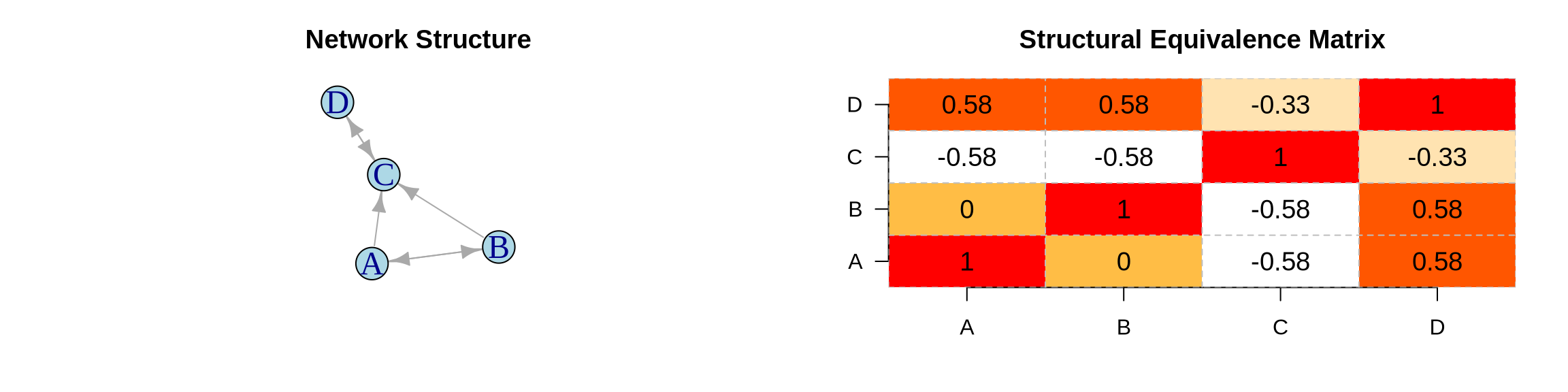
# Step 1: Compute Similarity Matrix (Correlation of tie patterns)
similarity <- cor(t(adj))  # Transpose to correlate rows
similarity[is.na(similarity)] <- 0  # Handle nodes with no ties

# Step 2: Hierarchical Clustering
dist_matrix <- as.dist(1 - similarity)  # Convert similarity to distance
hc <- hclust(dist_matrix, method = "ward.D2")
positions <- cutree(hc, k = 3)  # Cut into 3 positions

# Step 3: Create Blockmodel (Image Matrix)
n_pos <- max(positions)
blockmodel <- matrix(0, nrow = n_pos, ncol = n_pos)
for(i in 1:n_pos) {
  for(j in 1:n_pos) {
    block <- adj[positions == i, positions == j, drop=FALSE]
    if(length(block) > 0) blockmodel[i, j] <- mean(block)
  }
}

# Visualize the three outputs
par(mfrow=c(1,3), mar=c(4,4,3,2))

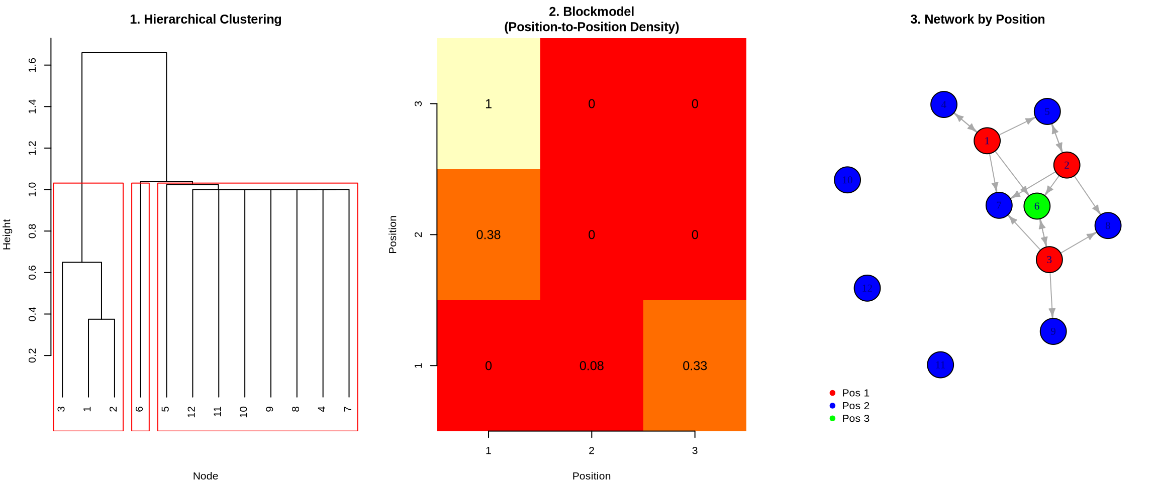
# 1. Dendrogram (Hierarchical Clustering)
plot(hc, main = "1. Hierarchical Clustering", xlab = "Node", sub = "", hang = -1)
rect.hclust(hc, k = 3, border = "red")

# 2. Image Matrix (Blockmodel)
image(1:n_pos, 1:n_pos, blockmodel, col = heat.colors(10), 
      main = "2. Blockmodel\n(Position-to-Position Density)",
      xlab = "Position", ylab = "Position", axes = FALSE)
axis(1, at = 1:n_pos); axis(2, at = 1:n_pos)
text(expand.grid(1:n_pos, 1:n_pos), labels = round(blockmodel, 2), cex = 1.2)

# 3. Network colored by position
V(g)$color <- c("red", "blue", "green")[positions]
plot(g, vertex.size = 20, edge.arrow.size = 0.5, 
     main = "3. Network by Position",
     vertex.label = 1:12)
legend("bottomleft", legend = paste("Pos", 1:3), 
       col = c("red", "blue", "green"), pch = 19, bty = "n")

Structural Equivalence: Definition

Two nodes are structurally equivalent if they have identical ties to the same alters

Example:

  • Node A connects to: {C, D, E}
  • Node B connects to: {C, D, E}
  • → A and B are structurally equivalent

Implication: They are substitutable - occupy the same position

Types of Equivalence

1. Structural Equivalence (Strict) - Two nodes are connected to the exact same other nodes. - Example: Two siblings who have the exact same parents and grandparents. - Business: Two customer service reps who handle the exact same set of tickets (rare).

2. Regular Equivalence (Functional) - Two nodes are connected to equivalent types of nodes. - Example: Two doctors. Dr. A treats Patient X; Dr. B treats Patient Y. They don’t know the same people, but they have the same relationship to their patients. - Business: Two department heads. They manage different teams, but structurally they are identical.

We typically use Structural Equivalence (via correlation) as a proxy for Regular Equivalence in dense networks.

Measuring Structural Equivalence

The Method: Use correlation to measure how similar two nodes’ tie patterns are.

  • High correlation (→ 1): Nodes connect to the same others → Structurally equivalent
  • Low correlation (→ 0 or negative): Nodes have different tie patterns → Different positions

Example Network: 4 nodes with directed ties

Interpretation

  • Nodes A & B: Correlation ≈ 1.0 → Highly equivalent (both connect to B, C)
  • Nodes C & D: Correlation ≈ 1.0 → Highly equivalent (both connect to C)
  • Nodes A & C: Correlation ≈ 0 → Not equivalent (different tie patterns)

Conclusion: We can group {A, B} into one position and {C, D} into another.

Summary: The Two Lenses

Feature Community Detection Role Analysis
Underlying Logic Cohesion (Adjacency) Equivalence (Similarity)
Key Metric Modularity Correlation / Euclidean Dist
Visual Result Clusters / Blobs Blockmodels / Hierarchies
Business Question “Who works with whom?” “Who does the same job?”
Typical Insight Silos, factions, teams Redundancy, hierarchy, gaps

Final Thought: A complete network analysis usually requires both. You want to know who is in the “Marketing Cluster” (Community) AND who is the “Bridge” (Role) within that cluster.

When Communities ≠ Positions

Example: Corporate structure

  • Communities: Departments (Marketing, R&D, Finance)
  • Positions: Ranks (Executives, Managers, Staff)

A Marketing Manager and an R&D Manager:

  • Different communities (different departments)
  • Same position (both supervise, both report up)