In this script, we create a bare-bone LDA model with Tomotopy. The final section of the script visualizes the LDA estimates with pyLDAvis.
Let’s start by importing the libraries we need for pre-processing (spaCy), estimation (tomotopy), data manipulation (NumPy and Pandas), and visualization tasks (Matplotlib, rich, pyLDAvis)
Python
Copy
>>> import os
>>> import numpy as np
>>> import matplotlib.pyplot as plt
>>> import pandas as pd
>>> import spacy
>>> import tomotopy as tp
>>> from rich.console import Console
>>> from rich.table import Table
>>> import pyLDAvis
We read the corpus of text, available in the GitHub repo under the sampleData directory. Here, I’m assuming the Python session is running under the topicModeling folder located in the same repo.
Python
Copy
>>> os.chdir("../sampleData/tripadvisorReviews")
>>> in_f = "hotel_reviews.csv"
>>> df = pd.read_csv((in_f))
Then, we pass the reviews, included in column ‘Review’ though a spaCy pipeline.
Python
Copy
>>> nlp = spacy.load("en_core_web_sm")
>>> docs_tokens, tmp_tokens = [], []
>>> for item in df.loc[:, "Review"].to_list():
tmp_tokens = [
token.lemma_
for token in nlp(item)
if not token.is_stop and not token.is_punct and not token.like_num
]
docs_tokens.append(tmp_tokens)
tmp_tokens = []
Now, our data look reasonably clean. Yet, there’s another step to carry out before running our LDA: we have to create a Tomotopy ‘corpus’ object, which we populate with the tokenized docs (see previous step).
Python
Copy
>>> corpus = tp.utils.Corpus(). # step 1: the empty corpus
>>> for item in docs_tokens: # step 2: we populate the corpus as we
corpus.add_doc(words=item). # iterate over tokenized docs
Hence, we can estimate an LDA model with an arbitrary number of topics (k = 10) over our object ‘corpus’ (see step 1). Note that Tomotopy trains an LDA model with an iterative approach to Gibbs-sampling. Hence, we have to specify the number of iterations (see step 2).
Python
Copy
>>> lda = tp.LDAModel(k=10, corpus=corpus) # step 1
>>> for i in range(0, 100, 10):
lda.train(10) # step 2
print("Iteration: {}\tLog-likelihood: {}".format(i, lda.ll_per_word))
Shell
Copy
Iteration: 0 Log-likelihood: -8.986793206269024
Iteration: 10 Log-likelihood: -8.683531180601642
Iteration: 20 Log-likelihood: -8.563040296738107
Iteration: 30 Log-likelihood: -8.489663788127347
Iteration: 40 Log-likelihood: -8.44406825673355
Iteration: 50 Log-likelihood: -8.415348844810286
Iteration: 60 Log-likelihood: -8.396785145655292
Iteration: 70 Log-likelihood: -8.384133225237559
Iteration: 80 Log-likelihood: -8.373994052744647
Iteration: 90 Log-likelihood: -8.363973922167325
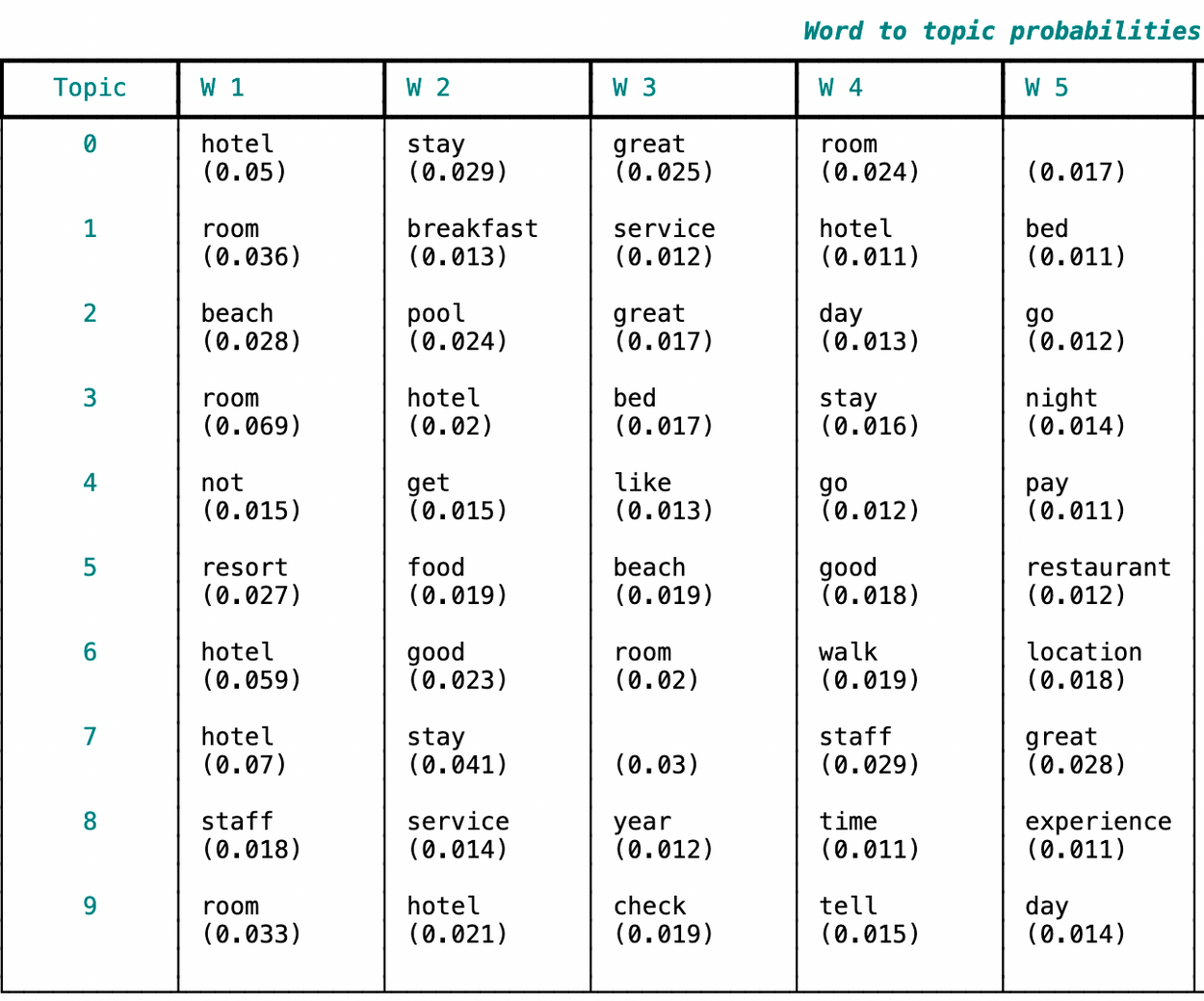
A critical part of a topic model’s output is the graph linking words with hidden topics. In the next block of code, we carry out the following tasks:
creation of a rich table (step 1)
retrieval of topic-word probabilities using lda.get_topic_words (step 2)
table display (step 3)
Python
Copy
>>> console = Console(). # step 1
>>> table = Table(
show_header=True,
header_style="cyan",
title="[bold] [cyan] Word to topic probabilities (top 10 words)[/cyan]",
width=150,
)
>>> table.add_column("Topic", justify="center", style="cyan", width=10)
>>> table.add_column("W 1", width=12)
>>> table.add_column("W 2", width=12)
>>> table.add_column("W 3", width=12)
>>> table.add_column("W 4", width=12)
>>> table.add_column("W 5", width=12)
>>> table.add_column("W 6", width=12)
>>> table.add_column("W 7", width=12)
>>> table.add_column("W 8", width=12)
>>> table.add_column("W 9", width=12)
>>> table.add_column("W 10", width=12)
>>> for k in range(lda.k): # step 2
values = []
for word, prob in lda.get_topic_words(k):
values.append("{}\n({})\n".format(word, str(np.round(prob, 3))))
table.add_row(
str(k),
values[0],
values[1],
values[2],
values[3],
values[4],
values[5],
values[6],
values[7],
values[8],
values[9],
)
>>> table
Here’s a portion of the table with the topic-word probabilities. Note the larger the probability the more strongly the association between a topic and a word. It’s customary to report the five or ten mostly associated words per topic.
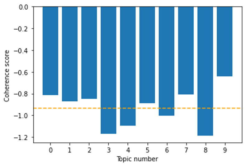
The statistical fit of a topic model can be assessed according to multiple metrics. The Coherence Score is one of the most popular metrics. Using the ‘get_score’ method over the a ‘Coherence’ class object (see step 1 and the Tomotopy’s coherence sub-module) it is possible to retrieve the average coherence score across topics or the coherence score of individual topics. See steps 2 and 3 respectively.
Python
Copy
>>> coh = tp.coherence.Coherence(lda, coherence="u_mass") # step 1
>>> average_coherence = coh.get_score() # step 2
>>> coherence_per_topic = [ # step 3
coh.get_score(topic_id=k) for k in range(lda.k)
]
The Coherence Score values associated with alternative models — i.e., models retaining different number of topics — can then be inspected visually using the following Matplotlib snippet.
Python
Copy
>>> fig = plt.figure()
>>> ax = fig.add_subplot(111)
>>> ax.bar(range(lda.k), coherence_per_topic)
>>> ax.set_xticks(range(lda.k))
>>> ax.set_xlabel("Topic number")
>>> ax.set_ylabel("Coherence score")
>>> plt.axhline(y=average_coherence, color="orange", linestyle="--")
>>> plt.show()
This snippet comes from the Python script “barebone_tomotopy.py”, hosted in the GitHub repo simoneSantoni/NLP-orgs-markets.