Oftentimes, we analyze vectors associated with entities such as companies and products. A way to get a better understanding of the meanings associated with a company or product is retrieving the neighbor vectors, that is, the vectors in the vicinity of the target one.
Let’s start by loading the libraries needed for this script.
Python
Copy
>>> import numpy as np
>>> import matplotlib.pyplot as plt
>>> from scipy.spatial.distance import cosine
>>> from sklearn.manifold import TSNE
>>> import seaborn as sns
>>> import gensim.downloader as api
>>> from gensim.models import Word2Vec
>>> import pandas as pd
We also define some custom colors to use in the following visualizations. The first one is the basic color, while the second and third were selected to create a triadic palette.
Python
Copy
>>> base_c = [i / 255 for i in [153, 0, 0]]
>>> tri_1_c = [i / 255 for i in [25, 196, 49]]
>>> tri_2_c = [i / 255 for i in [49, 25, 196]]
We borrow word2vec vectors from Genism.
Python
Copy
>>> wv = api.load("word2vec-google-news-300")
The set of target entities comprises three professional sport stars.
Python
Copy
>>> players = ["cristiano_ronaldo", "kobe_bryant", "tom_brady"]
For each entity, we retrieve the associated word vector.
Python
Copy
>>> vectors = [] # container
>>> for player in players:
try: # exception handling
artis_vector = wv[player]
vectors.append(artis_vector)
except:
print("vector not available for {}".format(artist))
Having retrieved the word vectors, one may want to visualize the semantic relationships among the three entities. To do that, we first reduce the dimensionality of the data using scikit-learn T-distributed Stochastic Neighbor Embedding.
Python
Copy
>>> tsne_model = TSNE(n_components=2) # we want 2D data
>>> coordinates = tsne_model.fit_transform(vectors) # the coordinates
>>> df = pd.DataFrame( # the DF with the data
{
"x": [x for x in coordinates[:, 0]],
"y": [y for y in coordinates[:, 1]],
"player": players,
}
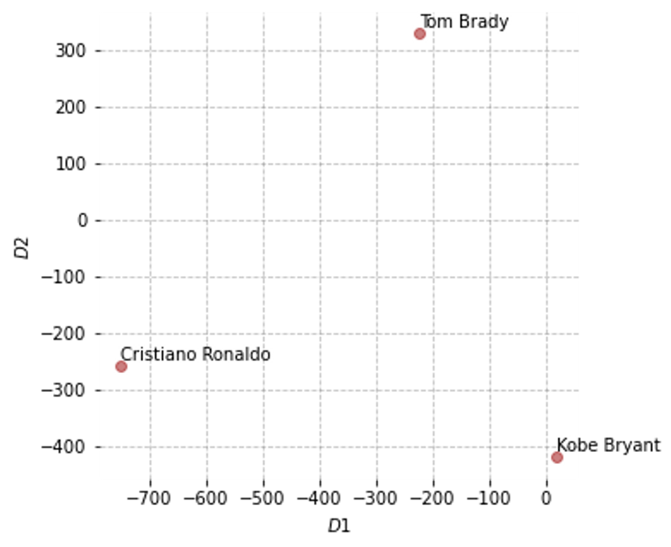
With Matplotlib, we create a scatter diagram illustrating the positions of the three players in the vector space (as represented by applying the word2vec algorithm over the Google News Corpus).
Python
Copy
>>> fig = plt.figuresize=(5, 5))
>>> ax = fig.add_subplot(1, 1, 1)
>>> plot = ax.scatter(df.x, df.y, marker="o", color=base_c, alpha=0.5)
>>> labels = []
>>> for player in players:
split = player.split("_")
split = [s.title() for s in split]
labels.append(" ".join(split))
>>> for i in range(len(df)):
ax.annotate("{}".format(labels[i]), (df.x[i], df.y[i] + 10))
>>> ax.spines["right"].set_visible(False)
>>> ax.spines["top"].set_visible(False)
>>> ax.spines["bottom"].set_visible(False)
>>> ax.spines["left"].set_visible(False)
>>> ax.set_xlabel(u"$D1$")
>>> ax.set_ylabel(u"$D2$")
>>> ax.grid(True, linestyle="--", color="grey", alpha=0.5)
>>> plt.show()
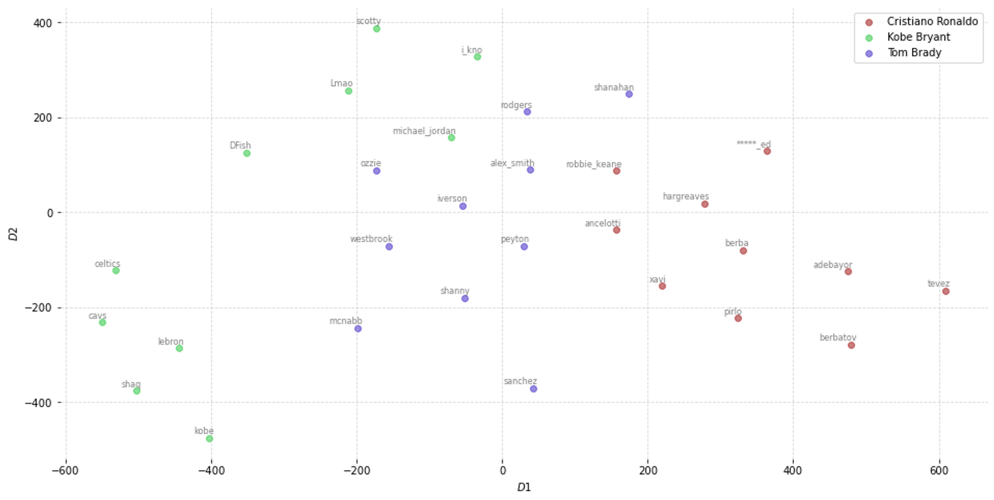
The following step consists of identifying the ten vectors that are most associated with each individual target words. To do that, we take advantage of the function “most_similar” included in the Gensim library. The below-display nested for loop iterates over the elements of the list “players” (step 1) and over the neighbor positions (step 2) to populate two containers: “word_clusters” has the neighbor words, while “embedding_clusters” the neighbor words’ embeddings.
Python
Copy
>>> embedding_clusters = []
>>> word_clusters = []
>>> for player in players: # step 1
embeddings = []
words = []
for similar_word, _ in wv.most_similar(player, topn=10): # step 2
words.append(similar_word)
embeddings.append(wv[similar_word])
embedding_clusters.append(embeddings)
word_clusters.append(words)
Similarly to what we’ve done for the previous scatter diagram, we use a dimensionality reduction approach to plot the positions of the neighbor words in the vector space.
Python
Copy
>>> tsne_model_en_2d = TSNE(
perplexity=15, n_components=2, init="pca", n_iter=3500, random_state=32
)
>>> embedding_clusters = np.array(embedding_clusters)
>>> n, m, k = embedding_clusters.shape
>>> embedding_clusters = embedding_clusters.reshape(n * m, k)
>>> tsne_output = tsne_model_en_2d.fit_transform(embedding_clusters)
>>> embeddings_en_2d = np.array(tsne_output).reshape(n, m, 2)
Now, it is possible to plot the data with Matplotlib.
Python
Copy
>>> fig = plt.figure(figsize=(16, 8))
>>> ax = fig.add_subplot(1, 1, 1)
>>> colors = [base_c, tri_1_c, tri_2_c]
>>> for label, embeddings, words, color in zip(
labels, embeddings_en_2d, word_clusters, colors
):
x = embeddings[:, 0]
y = embeddings[:, 1]
ax.scatter(x, y, c=color, label=label, alpha=0.5)
for i, word in enumerate(words):
plt.annotate(
word,
alpha=0.5,
xy=(x[i], y[i]),
xytext=(5, 2),
textcoords="offset points",
ha="right",
va="bottom",
size=8,
)
>>> ax.spines["right"].set_visible(False)
>>> ax.spines["top"].set_visible(False)
>>> ax.spines["bottom"].set_visible(False)
>>> ax.spines["left"].set_visible(False)
>>> ax.set_xlabel(u"$D1$")
>>> ax.set_ylabel(u"$D2$")
>>> plt.legend(loc="best")
>>> plt.grid(True, linestyle="--", alpha=0.5)
>>> plt.show(
This snippet comes from the Python script “neighbor_vectors.py”, hosted in the GitHub repo simoneSantoni/NLP-orgs-markets.