
In this script, we use scikit-learn to train a text classifier to discriminate between bad and good Tripadvisor reviews. The features for the text classifier are the topic-to-document probabilities from a pre-trained LDA model.
Let’s start by loading the libraries requires to implement the Python script. We need numPy and Pandas to carry out minimal data preparation activities. Regarding the NLP tasks, we use spaCy for pre-processing and Tomotopy for LDA modeling. Finally, we load the RidgeClassifier routines along with train_test_split utilities from the scikit-learn library.
Python
Copy
>>> import numpy as np
>>> import pandas as pd
>>> import matplotlib.pyplot as plt
>>> import seaborn as sns
>>> import spacy
>>> import tomotopy as tp
>>> from sklearn.model_selection import train_test_split
>>> from sklearn.linear_model import RidgeClassifier
We source the data from a local .csv file and display the key features.
Python
Copy
>>> df = pd.read_csv("../sampleData/tripadvisorReviews/hotel_reviews.csv")
>>> df.info()
Plain Text
Copy
<class 'pandas.core.frame.DataFrame'>
RangeIndex: 20491 entries, 0 to 20490
Data columns (total 2 columns):
# Column Non-Null Count Dtype
--- ------ -------------- -----
0 Review 20491 non-null object
1 Rating 20491 non-null int64
dtypes: int64(1), object(1)
memory usage: 320.3+ KB
Time top explore the data: we visualize the distribution of review across rating levels. Also, we make sure an observable review attribute such as text length does not vary ‘too much’ across rating levels.
Python
Copy
>>> sns.catplot(x="Rating", data=df, kind="count");
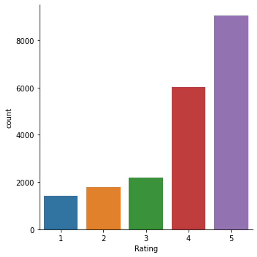
Distribution of reviews across rating levels
Python
Copy
>>> sns.violinplot(x="Rating", y=np.log(df.loc[:, "Review"].str.len()), data=df);
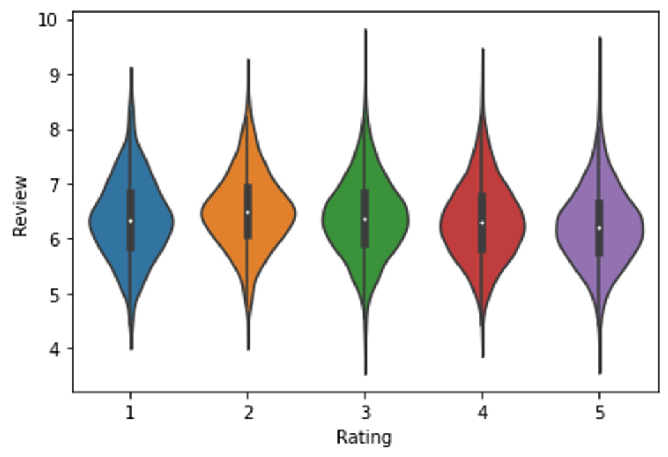
Distribution of review length across rating levels
The next step is creating review labels, say ‘bad’ and ‘good’, out of review ratings. As per prior literature on sentiment analysis, 1- and 2-star reviews are considered bad reviews, whereas 4- and 5-star reviews are considered good reviews.
Python
Copy
>>> df.loc[:, "label"] = np.nan
>>> df.loc[df["Rating"] < 3, "label"] = int(0)
>>> df.loc[df["Rating"] > 3, "label"] = int(1)
>>> sns.catplot(x="label", data=df.loc[df["label"].notnull()], kind="count");

Based on the distribution of the reviews across the ‘bad’ and ‘good’ classes, we create a matched dataset s with one ‘good review’ for any ‘bar review.
Python
Copy
>>> bad = df.loc[df["label"] == 0, ["Review", "label"]]
>>> good = df.loc[df["label"] == 1, ["Review", "label"]]
>>> good = good.sample(n=len(bad), random_state=42)
>>> s = pd.concat([bad, good])
Before running the LDA model, the sample reviews are pre-processed using a spaCy pipeline.
Python
Copy
>>> nlp = spacy.load("en_core_web_sm")
>>> docs = nlp.pipe(
s.loc[:, "Review"].str.lower(),
n_process=2,
batch_size=500,
disable=["tok2vec"],
)
>>> tkns_docs = []
>>> for doc in docs:
tmp = []
for token in doc:
if (
token.is_stop == False
and token.is_punct == False
and token.like_num == False
):
tmp.append(token.lemma_)
tkns_docs.append(tmp)
del tmp
The following steps consists of training and evaluating alternative LDA models, i.e., models retaining a different number of topics. Particularly, we sample 25 alternative models:
Python
Copy
>>> corpus = tp.utils.Corpus()
>>> for item in tkns_docs:
corpus.add_doc(words=item)
>>> mf = {}
>>> for i in range(10, 260, 10):
print(
">>> Working on the model with {} topics >>>\n".format(i),
flush=True
)
mdl = tp.LDAModel(k=i, corpus=corpus, min_df=5, rm_top=5, seed=42)
mdl.train(0)
for j in range(0, 1000, 10):
mdl.train(10)
print("Iteration: {}\tLog-likelihood: {}".format(j, mdl.ll_per_word))
coh = tp.coherence.Coherence(mdl, coherence="u_mass")
mf[i] = coh.get_score()
mdl.save("k_{}".format(i), True)
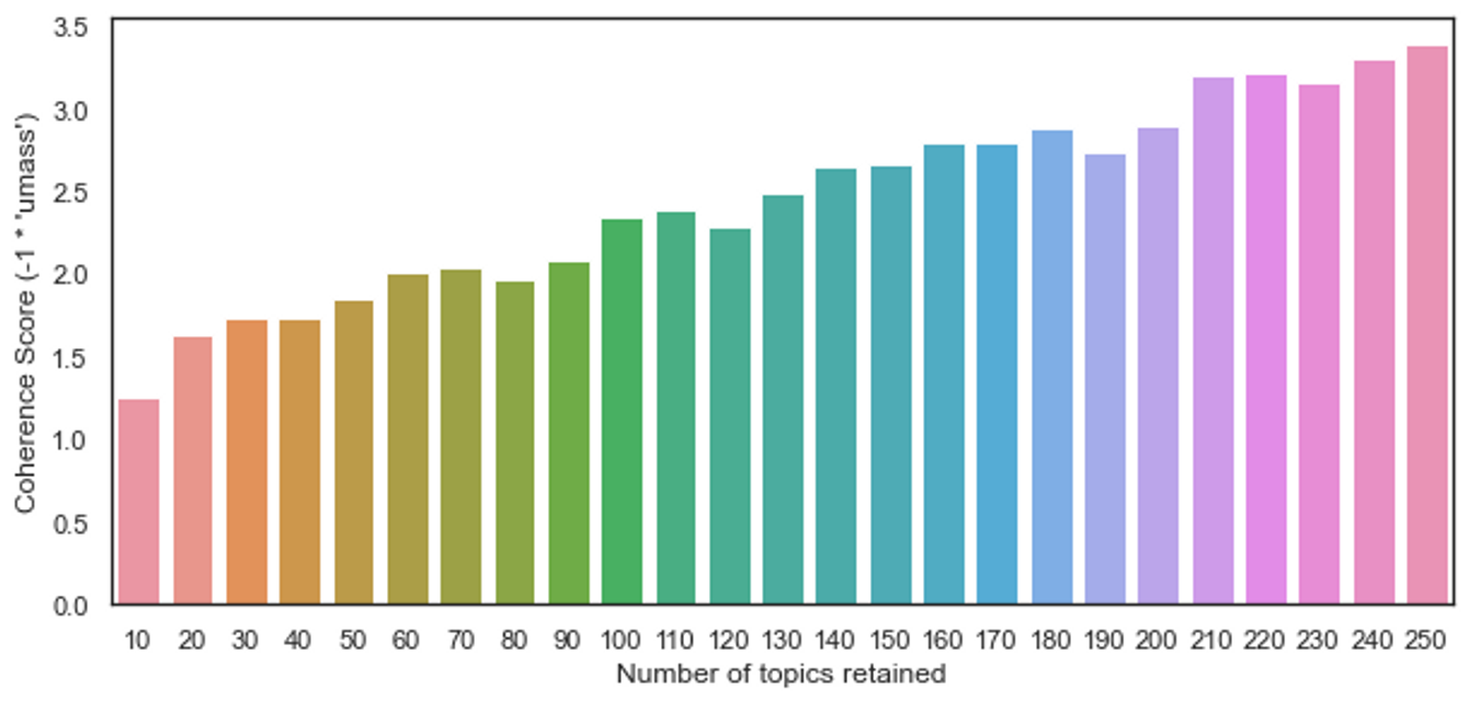
We identify the best fitting model on the basis of the Coherence score. The below displayed chart indicates the model with 250 topics has the largest Coherence score among the sample models.
Python
Copy
>>> fig = plt.figure(figsize=(10, 4.5))
>>> ax = fig.add_subplot(111)
>>> sns.barplot(x=list(mf.keys()), y=[-1*score for score in mf.values()], ax=ax)
>>> ax.set_xlabel("Number of topics retained")
>>> ax.set_ylabel("Coherence Score (-1 * 'umass')")
>>> plt.show()
The text classifier we want to train uses topic-to-document probabilities to predict review labels. Hence, we retrieve the estimates from the best fitting models (step 1), which we arrange into a Pandas DF (step 2).
Python
Copy
>>> best_mdl = tp.LDAModel.load("k_250"). # step 1
>>> td = pd.DataFrame( # step 2
np.stack([doc.get_topic_dist() for doc in best_mdl.docs]),
columns=["topic_{}".format(i + 1) for i in range(best_mdl.k)],
)
>>> td.info(verbose=True, null_counts=True)
Plain Text
Copy
<class 'pandas.core.frame.DataFrame'>
RangeIndex: 6428 entries, 0 to 6427
Data columns (total 250 columns):
# Column Non-Null Count Dtype
--- ------ -------------- -----
0 topic_1 6428 non-null float32
1 topic_2 6428 non-null float32
2 topic_3 6428 non-null float32
3 topic_4 6428 non-null float32
4 topic_5 6428 non-null float32
5 topic_6 6428 non-null float32
6 topic_7 6428 non-null float32
7 topic_8 6428 non-null float32
8 topic_9 6428 non-null float32
9 topic_10 6428 non-null float32
10 topic_11 6428 non-null float32
11 topic_12 6428 non-null float32
12 topic_13 6428 non-null float32
13 topic_14 6428 non-null float32
14 topic_15 6428 non-null float32
15 topic_16 6428 non-null float32
16 topic_17 6428 non-null float32
17 topic_18 6428 non-null float32
18 topic_19 6428 non-null float32
19 topic_20 6428 non-null float32
...
248 topic_249 6428 non-null float32
249 topic_250 6428 non-null float32
dtypes: float32(250)
memory usage: 6.1 MB
We are in the position to train a text classifier. In this example, scikit-learn’s RidgeClassifier is used. However, there are alternative estimators that could fit the task and the dataset at hand. First, we split the data into a trining and test sets.
Python
Copy
>>> X, y = td.loc[:,].values, s.loc[:, "label"].values
>>> X_train, X_test, y_train, y_test = train_test_split(
X,
y,
test_size=0.4,
random_state=0
)
Then, we create, train, and evaluate our model. Such a simple model achieves a satisfying level performance, ~ 0.91.
Python
Copy
>>> ridge_c = RidgeClassifier(alpha=0.1, random_state=0, fit_intercept=False)
>>> ridge_c.fit(X_train, y_train)
>>> ridge_c.score(X_test, y_test)
Plain Text
Copy
0.9094090202177294
This snippet comes from the Python script scikitlearn.ipynb, hosted in the GitHub repo simoneSantoni/NLP-orgs-markets.