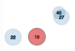
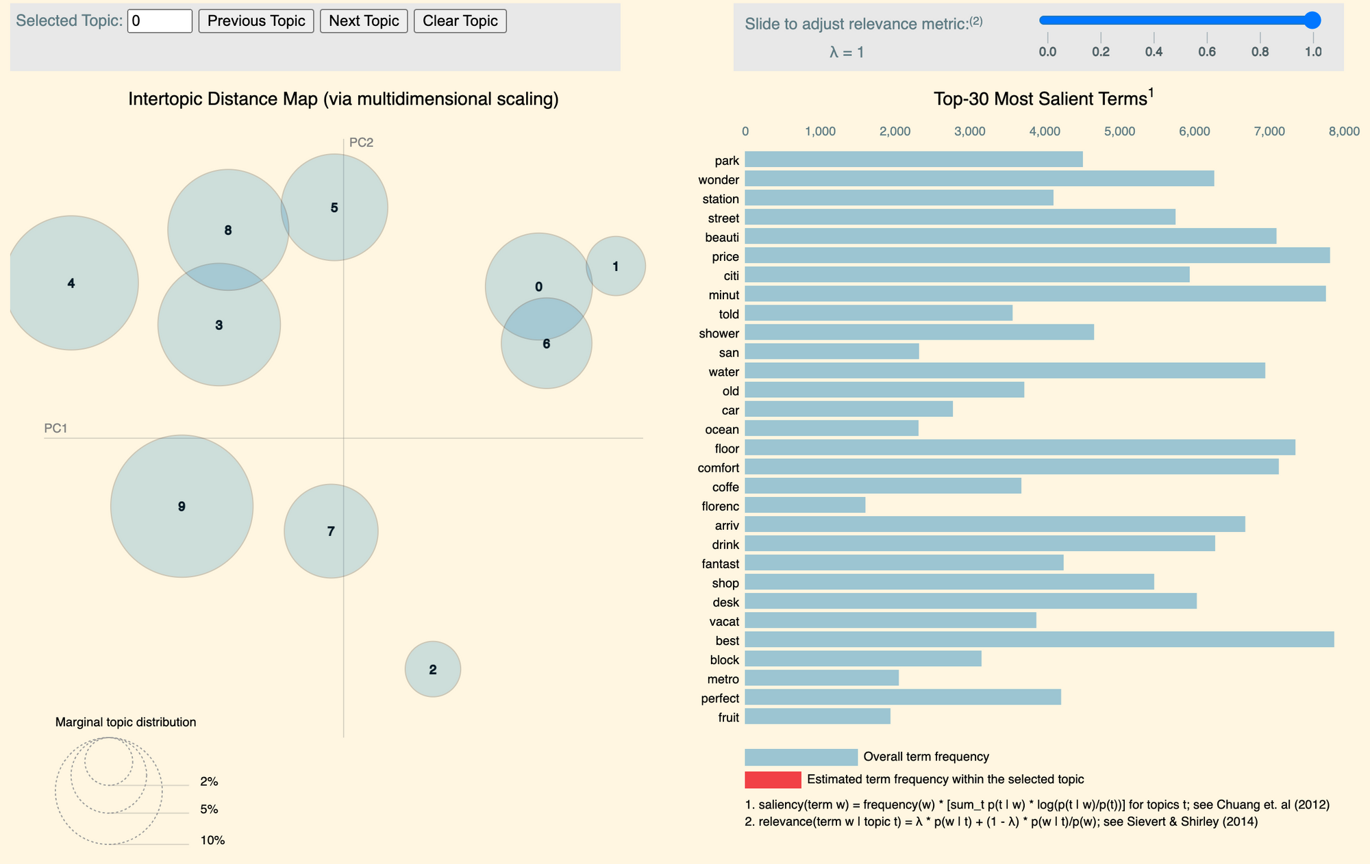
In this script, we visualize the outcome of a topic model. Particularly, we use pyLDAvis to produce an interactive plot showing:
the relative positions of the rendered topics
the associations between words and topics
word co-occurrences within topics
We will also use the tmplot library to create a table showing each document’s the most relevant words by topics. Let’s load the libraries we need then.
Python
Copy
>>> import nltk
>>> from nltk.corpus import stopwords
>>> import re
>>> import tomotopy as tp
>>> import pandas as pd
>>> import pyLDAvis
>>> import tmplot
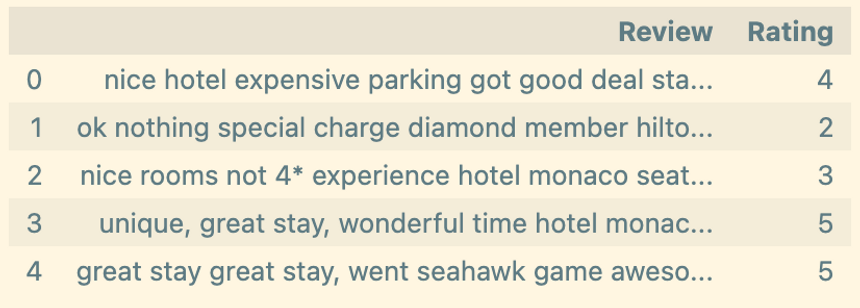
To produce some LDA estimates, we process ‘Tripadvisor corpus’ with Tomotopy. The data structure is fairly simple: each record contains a textual review and a rating.
Python
Copy
>>> df = pd.read_csv('../sampleData/tripadvisorReviews/hotel_reviews.csv')
>>> df.head()
To keep things simple, we create a tokenizer with NLTK (steps 1, 2, 3), which we pass to Tomotopy’s SimpleTokenizer, included in the utils module (step 4).
Python
Copy
>>> porter_stemmer = nltk.PorterStemmer().stem # step 1
>>> english_stops = set( # step 2
porter_stemmer(w) for w in stopwords.words('english')
)
>>> pat = re.compile('^[a-z]{2,}$') # step 3
>>> corpus = tp.utils.Corpus( # step 4
tokenizer=tp.utils.SimpleTokenizer(porter_stemmer),
stopwords=lambda x: x in english_stops or not pat.match(x)
)
The object corpus is a Tomotopy Corpus class object, which will we populate as follows.
Python
Copy
>>> reviews = df['Review'].tolist()
>>> corpus.process(doc.lower() for doc in reviews)
Having created the corpus of documents, we set the LDA model up. Note the number of topics retained is completely arbitrary — we just want to create sample estimates to plot here. The last two line print a minimal log concerning the corpus’ features.
Python
Copy
>>> mdl = tp.LDAModel(min_df=5, rm_top=40, k=10, corpus=corpus)
>>> mdl.train(0)
>>> print('Num docs:{}, Num Vocabs:{}, Total Words:{}'.format(
len(mdl.docs), len(mdl.used_vocabs), mdl.num_words
))
>>> print('Removed Top words: ', *mdl.removed_top_words)
We train the model using the ‘train’ method included in the LDAModel module.
Python
Copy
>>> for i in range(0, 1000, 20):
print('Iteration: {:04}, LL per word: {:.4}'.format(i, mdl.ll_per_word))
mdl.train(20)
>>> print('Iteration: {:04}, LL per word: {:.4}'.format(1000, mdl.ll_per_word))
>>> mdl.summary()
To create a pyLDAvis interactive plot, we have to manipulate the outcome of the LDA procedure. Specifically, pyLDAvis requires the following inputs:
the distribution of words over topics (step 1)
the distribution of topics over words (step 2)
the length of each document included in the corpus (step 3)
the vocabulary of words used in the LDA procedure (step 4)
the frequency of each word in the corpus (step 5)
Python
Copy
>>> topic_term_dists = np.stack( # step 1
[mdl.get_topic_word_dist(k) for k in range(mdl.k)]
)
>>> doc_topic_dists = np.stack( # step 2
[doc.get_topic_dist() for doc in mdl.docs]
)
>>> doc_topic_dists /= doc_topic_dists.sum(axis=1, keepdims=True)
>>> doc_lengths = np.array([len(doc.words) for doc in mdl.docs]) # step 3
>>> vocab = list(mdl.used_vocabs) # step 4
>>> term_frequency = mdl.used_vocab_freq # step 5
In the next step, we wrap these inputs in a using the ‘prepare’ method of pyLDAvis, creating a named tuple containing all the data structures required for the visualization. To preserve the match between the index of the topics in Tomotopy and the index of the topics visualized with pyLDAvis, it is advisable to set the option sort_topics == FALSE.
Python
Copy
>>> prepared_data = pyLDAvis.prepare(
topic_term_dists,
doc_topic_dists,
doc_lengths,
vocab,
term_frequency,
start_index=0,
sort_topics=False
)
We can now visualize and/or save the interactive plot as follows.
Python
Copy
>>> pyLDAvis.display(prepared_data)
>>> pyLDAvis.save_html(prepared_data, 'ldavis.html')
This snippet comes from the notebook “visualization.ipynb”, hosted in the GitHub repo simoneSantoni/NLP-orgs-markets.