---
title: "Apex Manufacturing: Structural Holes and Performance"
subtitle: "Week 10 - Case Analysis"
format:
html:
toc: true
toc-depth: 3
code-fold: false
code-tools: true
execute:
freeze: auto
jupyter: python3
---
## Introduction
This notebook analyzes the Apex Manufacturing case study, examining how network position shapes managerial performance and idea generation. We investigate the relationship between **structural holes** (gaps in network structure) and career outcomes (salary, evaluation, promotion) across 673 supply-chain managers.
### Research Questions
We address four key questions:
1. **Vision Advantage**: What network positions offer the greatest "vision advantage" for identifying good ideas, and why are managers with low constraint more likely to have their ideas valued?
2. **Opportunities and Risks**: How do structural holes between business units create both opportunities and risks for managers seeking to innovate?
3. **Organizational Silence**: Why do only 68% of managers respond to surveys about ideas, and what does this pattern reveal about network dynamics?
4. **Career Trajectories**: How do high-constraint vs. low-constraint managers differ in their career outcomes (salary, evaluation, promotion), and what mechanisms explain this gap?
### Data Structure
The dataset contains:
- **Nodes** (`nodes.csv`): 673 managers with attributes including rank, business unit, network constraint, and performance metrics
- **Edges** (`edges.csv`): 1,219 relationships between managers, weighted by interaction frequency
```{python}
#| label: setup
#| code-summary: "Import libraries"
import numpy as np
import pandas as pd
import networkx as nx
import matplotlib.pyplot as plt
import matplotlib.patches as mpatches
import seaborn as sns
from scipy import stats
import warnings
warnings.filterwarnings('ignore')

# Set random seed for reproducibility
np.random.seed(42)

# Set plotting style
sns.set_style("whitegrid")
plt.rcParams['figure.dpi'] = 100

print("Libraries loaded successfully")
print(f"NetworkX version: {nx.__version__}")
print(f"Pandas version: {pd.__version__}")
```
## 1. Data Loading and Network Construction
```{python}
#| label: load-data
# Load node data
nodes_df = pd.read_csv('../../../data/apex/nodes.csv')
print(f"Loaded {len(nodes_df)} managers")
print(f"\nNode attributes: {list(nodes_df.columns)}")
print(f"\nFirst few rows:")
nodes_df.head()
```
```{python}
#| label: load-edges
# Load edge data
edges_df = pd.read_csv('../../../data/apex/edges.csv')
print(f"\nLoaded {len(edges_df)} relationships")
print(f"\nEdge attributes: {list(edges_df.columns)}")
print(f"\nFirst few rows:")
edges_df.head()
```
```{python}
#| label: data-overview
# Key variable statistics
print("=" * 70)
print("DATA OVERVIEW")
print("=" * 70)

print("\n1. MANAGER RANKS")
print(nodes_df['rank'].value_counts().sort_index())

print("\n2. BUSINESS UNITS")
print(nodes_df['business_unit'].value_counts())

print("\n3. CONSTRAINT DISTRIBUTION")
print(nodes_df['constraint'].describe())

print("\n4. PERFORMANCE OUTCOMES")
print(f"\nEvaluation ratings:")
print(nodes_df['evaluation'].value_counts())
print(f"\nPromotion/Above Average: {nodes_df['promoted_or_aboveavg'].sum()} ({nodes_df['promoted_or_aboveavg'].mean()*100:.1f}%)")

print("\n5. IDEA GENERATION")
print(f"Responded to survey: {nodes_df['responded'].sum()} ({nodes_df['responded'].mean()*100:.1f}%)")
print(f"Expressed idea: {nodes_df['idea_expressed'].sum()} ({nodes_df[nodes_df['responded']==True]['idea_expressed'].mean()*100:.1f}% of respondents)")
print(f"Idea discussed: {nodes_df['idea_discussed'].sum()}")
print(f"Idea valued: {nodes_df[nodes_df['idea_discussed']==True]['idea_value'].notna().sum()}")
print(f"Idea dismissed: {nodes_df[nodes_df['idea_discussed']==True]['idea_dismissed'].sum()}")
```
```{python}
#| label: create-network
# Create NetworkX graph
G = nx.Graph()

# Add nodes with attributes
for _, row in nodes_df.iterrows():
    G.add_node(row['id'],
               rank=row['rank'],
               business_unit=row['business_unit'],
               constraint=row['constraint'],
               log_constraint=row['log_constraint'],
               degree=row['degree'],
               betweenness=row['betweenness'],
               evaluation=row['evaluation'],
               salary_resid=row['salary_resid'],
               promoted_or_aboveavg=row['promoted_or_aboveavg'],
               responded=row['responded'],
               idea_expressed=row['idea_expressed'],
               idea_value=row['idea_value'] if pd.notna(row['idea_value']) else None)

# Add edges with weights
for _, row in edges_df.iterrows():
    G.add_edge(row['source'], row['target'], weight=row['weight'])

print(f"Network created:")
print(f"  Nodes: {G.number_of_nodes()}")
print(f"  Edges: {G.number_of_edges()}")
print(f"  Density: {nx.density(G):.4f}")
print(f"  Connected: {nx.is_connected(G)}")
if nx.is_connected(G):
    print(f"  Average path length: {nx.average_shortest_path_length(G):.3f}")
```
## 2. Question 1: Vision Advantage and Constraint
**Question**: What network positions offer the greatest "vision advantage" for identifying good ideas, and why are managers with low constraint more likely to have their ideas valued?
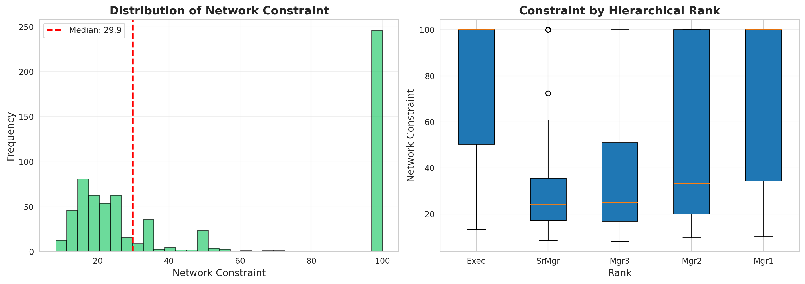
### 2.1 Constraint and Idea Quality
```{python}
#| label: q1-constraint-distribution
#| fig-cap: "Distribution of Burt's Network Constraint"
fig, axes = plt.subplots(1, 2, figsize=(14, 5))

# Histogram of constraint
axes[0].hist(nodes_df['constraint'], bins=30, edgecolor='black', alpha=0.7, color='#2ecc71')
axes[0].axvline(nodes_df['constraint'].median(), color='red', linestyle='--',
                linewidth=2, label=f'Median: {nodes_df["constraint"].median():.1f}')
axes[0].set_xlabel('Network Constraint', fontsize=12)
axes[0].set_ylabel('Frequency', fontsize=12)
axes[0].set_title('Distribution of Network Constraint', fontsize=14, fontweight='bold')
axes[0].legend()
axes[0].grid(alpha=0.3)

# Box plot by rank
rank_order = ['Exec', 'SrMgr', 'Mgr3', 'Mgr2', 'Mgr1']
nodes_df['rank'] = pd.Categorical(nodes_df['rank'], categories=rank_order, ordered=True)
nodes_df_sorted = nodes_df.sort_values('rank')

axes[1].boxplot([nodes_df_sorted[nodes_df_sorted['rank']==r]['constraint'].values
                 for r in rank_order],
                labels=rank_order, patch_artist=True)
axes[1].set_xlabel('Rank', fontsize=12)
axes[1].set_ylabel('Network Constraint', fontsize=12)
axes[1].set_title('Constraint by Hierarchical Rank', fontsize=14, fontweight='bold')
axes[1].grid(alpha=0.3, axis='y')

plt.tight_layout()
plt.show()

print("\nConstraint by Rank:")
print(nodes_df.groupby('rank')['constraint'].describe()[['mean', 'std', 'min', 'max']])
```
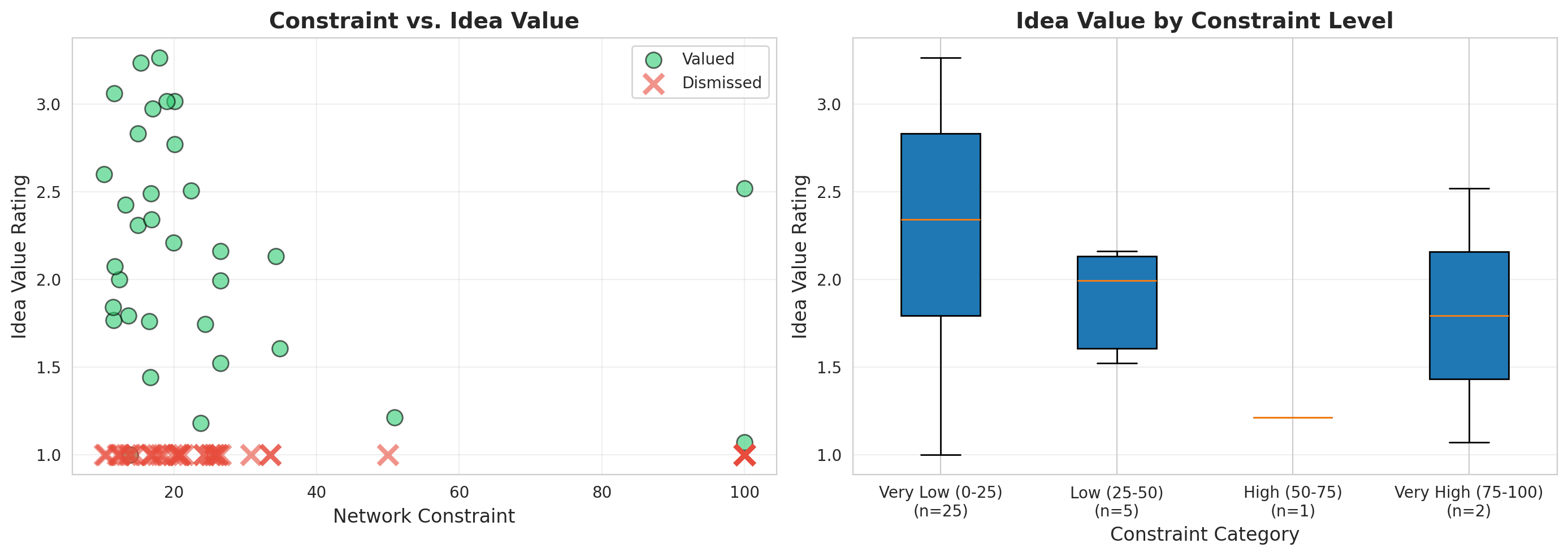
```{python}
#| label: q1-idea-quality
#| fig-cap: "Relationship between Constraint and Idea Value"
# Filter to managers who expressed ideas that were discussed
idea_managers = nodes_df[nodes_df['idea_discussed'] == True].copy()
print(f"Managers whose ideas were discussed: {len(idea_managers)}")

# Create constraint categories
idea_managers['constraint_category'] = pd.cut(idea_managers['constraint'],
                                               bins=[0, 25, 50, 75, 100],
                                               labels=['Very Low (0-25)', 'Low (25-50)',
                                                      'High (50-75)', 'Very High (75-100)'])

fig, axes = plt.subplots(1, 2, figsize=(14, 5))

# Scatter plot: constraint vs. idea value
valued = idea_managers[idea_managers['idea_dismissed'] == False]
dismissed = idea_managers[idea_managers['idea_dismissed'] == True]

axes[0].scatter(valued['constraint'], valued['idea_value'],
               alpha=0.6, s=100, color='#2ecc71', label='Valued', edgecolors='black')
axes[0].scatter(dismissed['constraint'], [1.0] * len(dismissed),
               alpha=0.6, color='#e74c3c', marker='x', s=150,
               linewidths=3, label='Dismissed')
axes[0].set_xlabel('Network Constraint', fontsize=12)
axes[0].set_ylabel('Idea Value Rating', fontsize=12)
axes[0].set_title('Constraint vs. Idea Value', fontsize=14, fontweight='bold')
axes[0].legend()
axes[0].grid(alpha=0.3)

# Box plot: idea value by constraint category
value_data = []
labels = []
for cat in ['Very Low (0-25)', 'Low (25-50)', 'High (50-75)', 'Very High (75-100)']:
    data = valued[valued['constraint_category'] == cat]['idea_value'].dropna()
    if len(data) > 0:
        value_data.append(data.values)
        labels.append(f"{cat}\n(n={len(data)})")

axes[1].boxplot(value_data, labels=labels, patch_artist=True)
axes[1].set_xlabel('Constraint Category', fontsize=12)
axes[1].set_ylabel('Idea Value Rating', fontsize=12)
axes[1].set_title('Idea Value by Constraint Level', fontsize=14, fontweight='bold')
axes[1].grid(alpha=0.3, axis='y')

plt.tight_layout()
plt.show()

# Statistical analysis
print("\n" + "=" * 70)
print("VISION ADVANTAGE ANALYSIS")
print("=" * 70)

print("\nIdea Value by Constraint:")
print(idea_managers.groupby('constraint_category')['idea_value'].agg(['count', 'mean', 'std']))

print("\nDismissal Rate by Constraint:")
dismissal_by_constraint = idea_managers.groupby('constraint_category')['idea_dismissed'].agg(['sum', 'count', 'mean'])
dismissal_by_constraint.columns = ['Dismissed', 'Total', 'Dismissal_Rate']
print(dismissal_by_constraint)

# Correlation
corr, pval = stats.spearmanr(valued['constraint'], valued['idea_value'], nan_policy='omit')
print(f"\nSpearman correlation (Constraint vs. Value): r = {corr:.3f}, p = {pval:.3f}")
```
### 2.2 Key Findings: Vision Advantage
```{python}
#| label: q1-summary
print("=" * 70)
print("KEY FINDINGS: VISION ADVANTAGE")
print("=" * 70)

# Calculate key metrics
low_constraint = nodes_df[nodes_df['constraint'] < 50]
high_constraint = nodes_df[nodes_df['constraint'] >= 50]

print(f"\n1. CONSTRAINT DISTRIBUTION")
print(f"   Low constraint (<50): {len(low_constraint)} managers ({len(low_constraint)/len(nodes_df)*100:.1f}%)")
print(f"   High constraint (≥50): {len(high_constraint)} managers ({len(high_constraint)/len(nodes_df)*100:.1f}%)")
print(f"   Mean constraint: {nodes_df['constraint'].mean():.2f}")
print(f"   Median constraint: {nodes_df['constraint'].median():.2f}")

print(f"\n2. IDEA QUALITY BY CONSTRAINT")
low_c_ideas = idea_managers[idea_managers['constraint'] < 50]
high_c_ideas = idea_managers[idea_managers['constraint'] >= 50]

if len(low_c_ideas) > 0 and len(high_c_ideas) > 0:
    print(f"   Low constraint managers:")
    print(f"     - Average idea value: {low_c_ideas['idea_value'].mean():.2f}")
    print(f"     - Dismissal rate: {low_c_ideas['idea_dismissed'].mean()*100:.1f}%")
    print(f"   High constraint managers:")
    print(f"     - Average idea value: {high_c_ideas['idea_value'].mean():.2f}")
    print(f"     - Dismissal rate: {high_c_ideas['idea_dismissed'].mean()*100:.1f}%")

print(f"\n3. INTERPRETATION")
print(f"   → Managers in low-constraint positions span structural holes")
print(f"   → Access to diverse, non-redundant information sources")
print(f"   → Greater exposure to novel ideas across business units")
print(f"   → Better positioned to synthesize and broker ideas")
```
## 3. Question 2: Opportunities and Risks of Structural Holes
**Question**: How do structural holes between business units create both opportunities and risks for managers seeking to innovate?
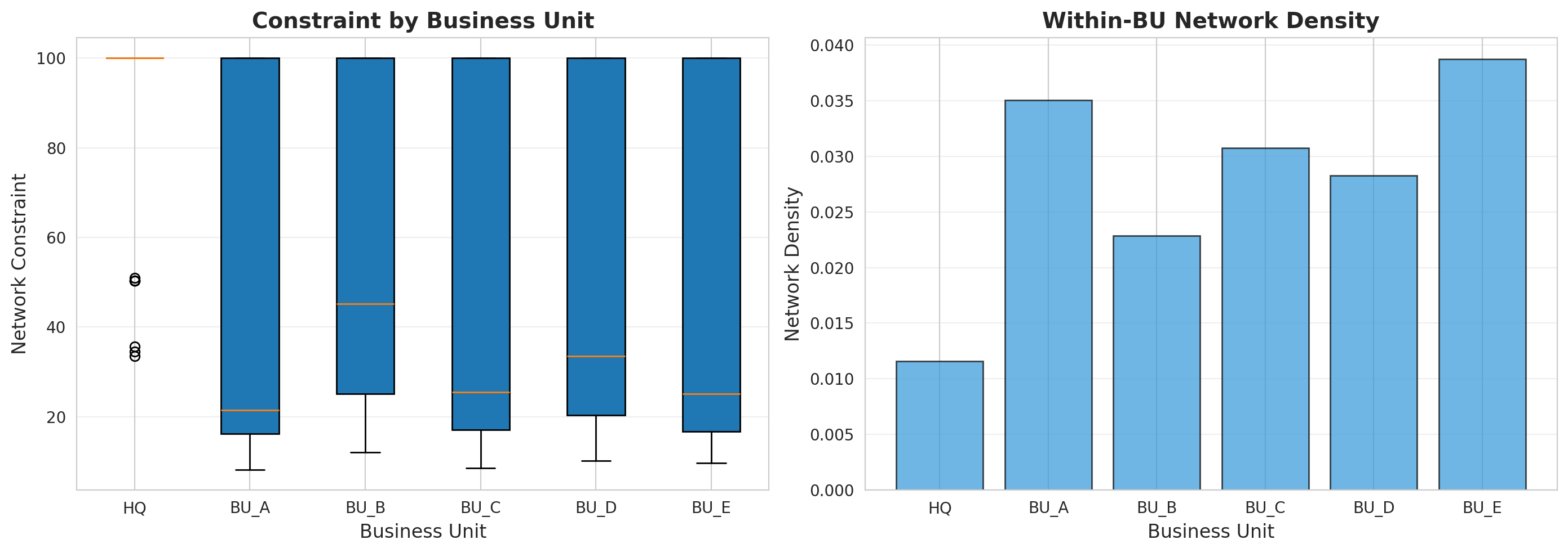
### 3.1 Business Unit Analysis
```{python}
#| label: q2-bu-structure
#| fig-cap: "Network structure across business units"
# Cross-business unit connections
within_bu = edges_df[edges_df['bu_u'] == edges_df['bu_v']]
cross_bu = edges_df[edges_df['bu_u'] != edges_df['bu_v']]

print("Business Unit Network Structure:")
print(f"  Within-BU ties: {len(within_bu)} ({len(within_bu)/len(edges_df)*100:.1f}%)")
print(f"  Cross-BU ties: {len(cross_bu)} ({len(cross_bu)/len(edges_df)*100:.1f}%)")

# Constraint by business unit
fig, axes = plt.subplots(1, 2, figsize=(14, 5))

# Constraint distribution by BU
bu_order = ['HQ', 'BU_A', 'BU_B', 'BU_C', 'BU_D', 'BU_E']
axes[0].boxplot([nodes_df[nodes_df['business_unit']==bu]['constraint'].values
                 for bu in bu_order],
                labels=bu_order, patch_artist=True)
axes[0].set_xlabel('Business Unit', fontsize=12)
axes[0].set_ylabel('Network Constraint', fontsize=12)
axes[0].set_title('Constraint by Business Unit', fontsize=14, fontweight='bold')
axes[0].grid(alpha=0.3, axis='y')

# Network density by BU
bu_networks = {}
bu_densities = {}
for bu in bu_order:
    bu_nodes = nodes_df[nodes_df['business_unit'] == bu]['id'].tolist()
    bu_subgraph = G.subgraph(bu_nodes)
    bu_networks[bu] = bu_subgraph
    bu_densities[bu] = nx.density(bu_subgraph) if len(bu_nodes) > 1 else 0

axes[1].bar(bu_order, [bu_densities[bu] for bu in bu_order],
           color='#3498db', edgecolor='black', alpha=0.7)
axes[1].set_xlabel('Business Unit', fontsize=12)
axes[1].set_ylabel('Network Density', fontsize=12)
axes[1].set_title('Within-BU Network Density', fontsize=14, fontweight='bold')
axes[1].grid(alpha=0.3, axis='y')

plt.tight_layout()
plt.show()

print("\nBusiness Unit Statistics:")
for bu in bu_order:
    bu_data = nodes_df[nodes_df['business_unit'] == bu]
    print(f"\n{bu}:")
    print(f"  Managers: {len(bu_data)}")
    print(f"  Mean constraint: {bu_data['constraint'].mean():.2f}")
    print(f"  Mean degree: {bu_data['degree'].mean():.2f}")
    print(f"  Network density: {bu_densities[bu]:.4f}")
```
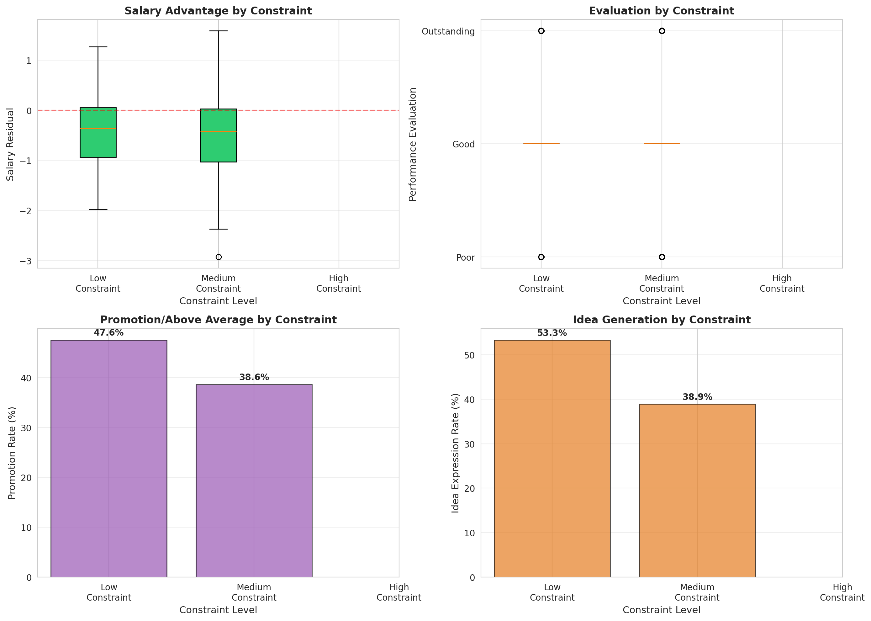
### 3.2 Opportunities: Brokerage Benefits
```{python}
#| label: q2-opportunities
#| fig-cap: "Performance benefits of low constraint (brokerage)"
# Create constraint terciles (due to many duplicate values at constraint=100, quartiles don't work well)
nodes_df['constraint_tercile_num'] = pd.qcut(nodes_df['constraint'], q=3, labels=False, duplicates='drop')
# Map to readable labels
tercile_labels = {0: 'Low', 1: 'Medium', 2: 'High'}
nodes_df['constraint_tercile'] = nodes_df['constraint_tercile_num'].map(tercile_labels)

fig, axes = plt.subplots(2, 2, figsize=(14, 10))

tercile_order = ['Low', 'Medium', 'High']

# 1. Salary residual by constraint tercile
salary_data = [nodes_df[nodes_df['constraint_tercile']==t]['salary_resid'].values
               for t in tercile_order]
bp1 = axes[0,0].boxplot(salary_data, labels=['Low\nConstraint', 'Medium\nConstraint', 'High\nConstraint'],
                        patch_artist=True)
for patch in bp1['boxes']:
    patch.set_facecolor('#2ecc71')
axes[0,0].axhline(0, color='red', linestyle='--', alpha=0.5)
axes[0,0].set_xlabel('Constraint Level', fontsize=11)
axes[0,0].set_ylabel('Salary Residual', fontsize=11)
axes[0,0].set_title('Salary Advantage by Constraint', fontsize=12, fontweight='bold')
axes[0,0].grid(alpha=0.3, axis='y')

# 2. Evaluation by constraint tercile
eval_mapping = {'Poor': 1, 'Good': 2, 'Outstanding': 3}
nodes_df['eval_numeric'] = nodes_df['evaluation'].map(eval_mapping)
eval_data = [nodes_df[nodes_df['constraint_tercile']==t]['eval_numeric'].values
             for t in tercile_order]
bp2 = axes[0,1].boxplot(eval_data, labels=['Low\nConstraint', 'Medium\nConstraint', 'High\nConstraint'],
                        patch_artist=True)
for patch in bp2['boxes']:
    patch.set_facecolor('#3498db')
axes[0,1].set_yticks([1, 2, 3])
axes[0,1].set_yticklabels(['Poor', 'Good', 'Outstanding'])
axes[0,1].set_xlabel('Constraint Level', fontsize=11)
axes[0,1].set_ylabel('Performance Evaluation', fontsize=11)
axes[0,1].set_title('Evaluation by Constraint', fontsize=12, fontweight='bold')
axes[0,1].grid(alpha=0.3, axis='y')

# 3. Promotion rate by constraint tercile
promo_rates = nodes_df.groupby('constraint_tercile')['promoted_or_aboveavg'].agg(['sum', 'count', 'mean'])
promo_rates = promo_rates.reindex(tercile_order)
axes[1,0].bar(range(3), promo_rates['mean'].values * 100,
             color='#9b59b6', edgecolor='black', alpha=0.7)
axes[1,0].set_xticks(range(3))
axes[1,0].set_xticklabels(['Low\nConstraint', 'Medium\nConstraint', 'High\nConstraint'])
axes[1,0].set_xlabel('Constraint Level', fontsize=11)
axes[1,0].set_ylabel('Promotion Rate (%)', fontsize=11)
axes[1,0].set_title('Promotion/Above Average by Constraint', fontsize=12, fontweight='bold')
axes[1,0].grid(alpha=0.3, axis='y')
for i, v in enumerate(promo_rates['mean'].values * 100):
    axes[1,0].text(i, v + 1, f'{v:.1f}%', ha='center', fontweight='bold')

# 4. Idea expression rate by constraint tercile
responded_df = nodes_df[nodes_df['responded'] == True].copy()
responded_df['constraint_tercile_num'] = pd.qcut(responded_df['constraint'], q=3, labels=False, duplicates='drop')
# Map to readable labels
responded_df['constraint_tercile'] = responded_df['constraint_tercile_num'].map(tercile_labels)
idea_rates = responded_df.groupby('constraint_tercile')['idea_expressed'].agg(['sum', 'count', 'mean'])
idea_rates = idea_rates.reindex(tercile_order)
axes[1,1].bar(range(3), idea_rates['mean'].values * 100,
             color='#e67e22', edgecolor='black', alpha=0.7)
axes[1,1].set_xticks(range(3))
axes[1,1].set_xticklabels(['Low\nConstraint', 'Medium\nConstraint', 'High\nConstraint'])
axes[1,1].set_xlabel('Constraint Level', fontsize=11)
axes[1,1].set_ylabel('Idea Expression Rate (%)', fontsize=11)
axes[1,1].set_title('Idea Generation by Constraint', fontsize=12, fontweight='bold')
axes[1,1].grid(alpha=0.3, axis='y')
for i, v in enumerate(idea_rates['mean'].values * 100):
    axes[1,1].text(i, v + 1, f'{v:.1f}%', ha='center', fontweight='bold')

plt.tight_layout()
plt.show()
```
### 3.3 Risks: Costs of Brokerage
```{python}
#| label: q2-risks
print("=" * 70)
print("OPPORTUNITIES AND RISKS OF STRUCTURAL HOLES")
print("=" * 70)

print("\n1. OPPORTUNITIES (Benefits of Low Constraint):")
low_tercile = nodes_df[nodes_df['constraint_tercile'] == 'Low']
high_tercile = nodes_df[nodes_df['constraint_tercile'] == 'High']

print(f"\n   Salary Advantage:")
print(f"   - Low constraint tercile: ${low_tercile['salary_resid'].mean():.2f} residual")
print(f"   - High constraint tercile: ${high_tercile['salary_resid'].mean():.2f} residual")
print(f"   - Difference: ${low_tercile['salary_resid'].mean() - high_tercile['salary_resid'].mean():.2f}")

print(f"\n   Promotion Rate:")
print(f"   - Low constraint tercile: {low_tercile['promoted_or_aboveavg'].mean()*100:.1f}%")
print(f"   - High constraint tercile: {high_tercile['promoted_or_aboveavg'].mean()*100:.1f}%")

print(f"\n   Outstanding Evaluations:")
low_outstanding = (low_tercile['evaluation'] == 'Outstanding').mean()
high_outstanding = (high_tercile['evaluation'] == 'Outstanding').mean()
print(f"   - Low constraint tercile: {low_outstanding*100:.1f}%")
print(f"   - High constraint tercile: {high_outstanding*100:.1f}%")

print("\n2. RISKS (Challenges of Low Constraint):")

# Cross-BU managers likely have lower constraint
cross_bu_managers = nodes_df[nodes_df['id'].isin(
    edges_df[edges_df['bu_u'] != edges_df['bu_v']]['source'].unique()
)]

print(f"\n   Spanning Business Units:")
print(f"   - Managers with cross-BU ties: {len(cross_bu_managers)}")
print(f"   - Mean constraint: {cross_bu_managers['constraint'].mean():.2f}")
print(f"   - [Risk] Potential for role conflict and competing demands")

# Isolates
isolates = nodes_df[nodes_df['degree'] == 0]
print(f"\n   Social Isolation:")
print(f"   - Managers with NO connections: {len(isolates)} ({len(isolates)/len(nodes_df)*100:.1f}%)")
print(f"   - Mean constraint of isolates: {isolates['constraint'].mean():.2f}")
print(f"   - [Risk] Complete disconnection despite structural opportunity")

print("\n3. THE BROKERAGE PARADOX:")
print(f"   → Low constraint = access to diverse information (opportunity)")
print(f"   → But also = lack of strong embedded ties (risk)")
print(f"   → Brokerage requires active effort and social skill")
print(f"   → Not all managers in structural holes realize the potential")
```
## 4. Question 3: Organizational Silence
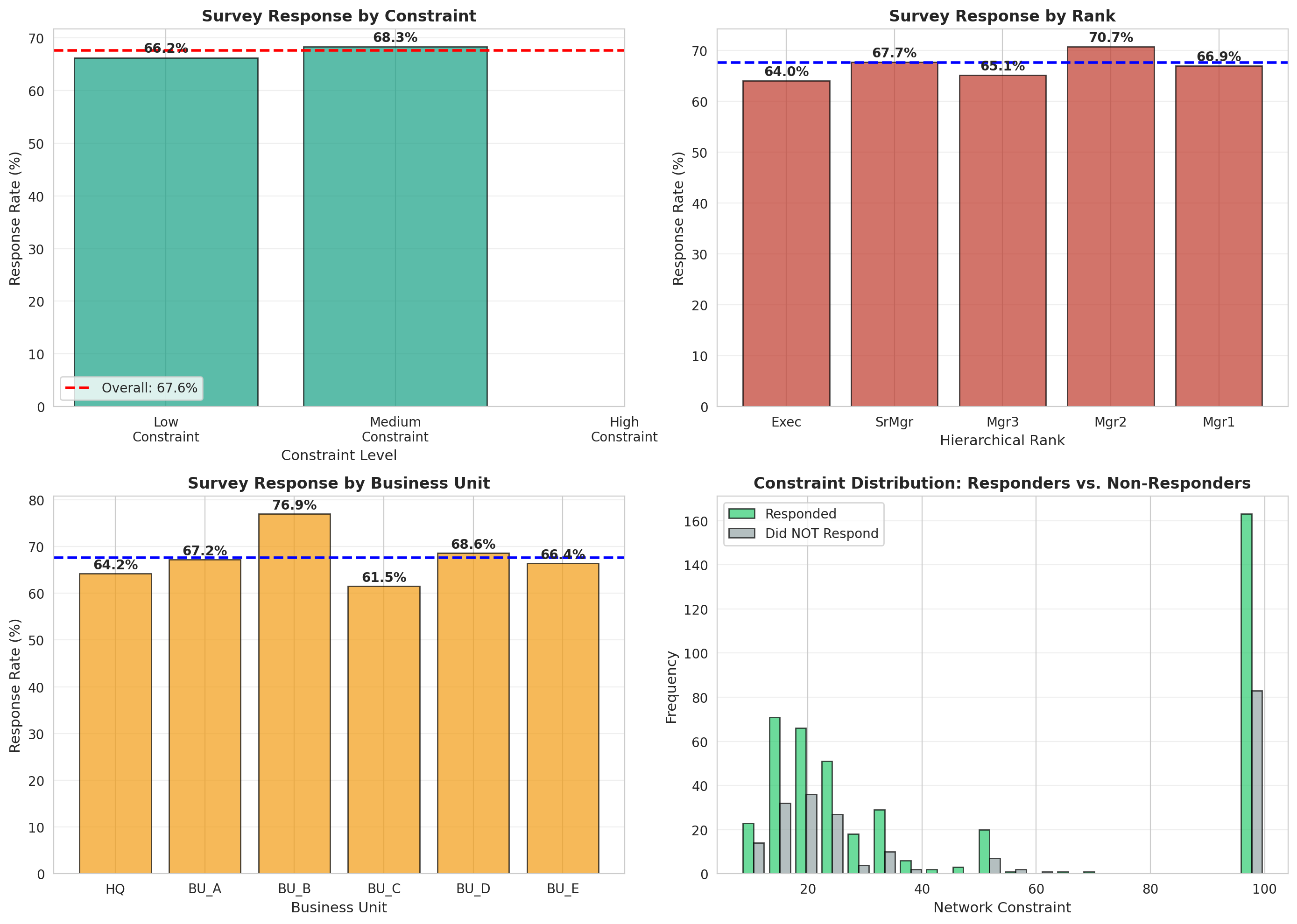
**Question**: Why do only 68% of managers respond to surveys about ideas, and what does this pattern of "organizational silence" reveal about network dynamics?
```{python}
#| label: q3-response-patterns
#| fig-cap: "Survey response patterns and organizational silence"
# Response statistics
total_managers = len(nodes_df)
responded = nodes_df['responded'].sum()
response_rate = responded / total_managers * 100

print("=" * 70)
print("ORGANIZATIONAL SILENCE ANALYSIS")
print("=" * 70)

print(f"\n1. OVERALL RESPONSE PATTERNS")
print(f"   Total managers: {total_managers}")
print(f"   Responded to survey: {responded} ({response_rate:.1f}%)")
print(f"   Did NOT respond: {total_managers - responded} ({100-response_rate:.1f}%)")

# Response by constraint
fig, axes = plt.subplots(2, 2, figsize=(14, 10))

# 1. Response rate by constraint tercile
response_by_t = nodes_df.groupby('constraint_tercile')['responded'].agg(['sum', 'count', 'mean'])
response_by_t = response_by_t.reindex(tercile_order)
axes[0,0].bar(range(3), response_by_t['mean'].values * 100,
             color='#16a085', edgecolor='black', alpha=0.7)
axes[0,0].axhline(response_rate, color='red', linestyle='--', linewidth=2,
                 label=f'Overall: {response_rate:.1f}%')
axes[0,0].set_xticks(range(3))
axes[0,0].set_xticklabels(['Low\nConstraint', 'Medium\nConstraint', 'High\nConstraint'])
axes[0,0].set_xlabel('Constraint Level', fontsize=11)
axes[0,0].set_ylabel('Response Rate (%)', fontsize=11)
axes[0,0].set_title('Survey Response by Constraint', fontsize=12, fontweight='bold')
axes[0,0].legend()
axes[0,0].grid(alpha=0.3, axis='y')
for i, v in enumerate(response_by_t['mean'].values * 100):
    axes[0,0].text(i, v + 1, f'{v:.1f}%', ha='center', fontweight='bold')

# 2. Response rate by rank
response_by_rank = nodes_df.groupby('rank')['responded'].agg(['sum', 'count', 'mean'])
response_by_rank = response_by_rank.reindex(rank_order)
axes[0,1].bar(range(len(rank_order)), response_by_rank['mean'].values * 100,
             color='#c0392b', edgecolor='black', alpha=0.7)
axes[0,1].axhline(response_rate, color='blue', linestyle='--', linewidth=2)
axes[0,1].set_xticks(range(len(rank_order)))
axes[0,1].set_xticklabels(rank_order)
axes[0,1].set_xlabel('Hierarchical Rank', fontsize=11)
axes[0,1].set_ylabel('Response Rate (%)', fontsize=11)
axes[0,1].set_title('Survey Response by Rank', fontsize=12, fontweight='bold')
axes[0,1].grid(alpha=0.3, axis='y')
for i, v in enumerate(response_by_rank['mean'].values * 100):
    axes[0,1].text(i, v + 1, f'{v:.1f}%', ha='center', fontweight='bold')

# 3. Response rate by business unit
response_by_bu = nodes_df.groupby('business_unit')['responded'].agg(['sum', 'count', 'mean'])
response_by_bu = response_by_bu.reindex(bu_order)
axes[1,0].bar(range(len(bu_order)), response_by_bu['mean'].values * 100,
             color='#f39c12', edgecolor='black', alpha=0.7)
axes[1,0].axhline(response_rate, color='blue', linestyle='--', linewidth=2)
axes[1,0].set_xticks(range(len(bu_order)))
axes[1,0].set_xticklabels(bu_order)
axes[1,0].set_xlabel('Business Unit', fontsize=11)
axes[1,0].set_ylabel('Response Rate (%)', fontsize=11)
axes[1,0].set_title('Survey Response by Business Unit', fontsize=12, fontweight='bold')
axes[1,0].grid(alpha=0.3, axis='y')
for i, v in enumerate(response_by_bu['mean'].values * 100):
    axes[1,0].text(i, v + 1, f'{v:.1f}%', ha='center', fontweight='bold')

# 4. Response vs. Non-response: Constraint comparison
responders = nodes_df[nodes_df['responded'] == True]['constraint']
non_responders = nodes_df[nodes_df['responded'] == False]['constraint']
axes[1,1].hist([responders, non_responders], bins=20, alpha=0.7,
              label=['Responded', 'Did NOT Respond'],
              color=['#2ecc71', '#95a5a6'], edgecolor='black')
axes[1,1].set_xlabel('Network Constraint', fontsize=11)
axes[1,1].set_ylabel('Frequency', fontsize=11)
axes[1,1].set_title('Constraint Distribution: Responders vs. Non-Responders',
                    fontsize=12, fontweight='bold')
axes[1,1].legend()
axes[1,1].grid(alpha=0.3, axis='y')

plt.tight_layout()
plt.show()
```
```{python}
#| label: q3-silence-mechanisms
print("\n2. NETWORK POSITION AND VOICE")

responders = nodes_df[nodes_df['responded'] == True]
non_responders = nodes_df[nodes_df['responded'] == False]

print(f"\n   Responders (n={len(responders)}):")
print(f"   - Mean constraint: {responders['constraint'].mean():.2f}")
print(f"   - Mean degree: {responders['degree'].mean():.2f}")
print(f"   - Mean betweenness: {responders['betweenness'].mean():.4f}")

print(f"\n   Non-Responders (n={len(non_responders)}):")
print(f"   - Mean constraint: {non_responders['constraint'].mean():.2f}")
print(f"   - Mean degree: {non_responders['degree'].mean():.2f}")
print(f"   - Mean betweenness: {non_responders['betweenness'].mean():.4f}")

# Statistical test
t_stat, p_val = stats.ttest_ind(responders['constraint'], non_responders['constraint'])
print(f"\n   T-test (Constraint): t = {t_stat:.3f}, p = {p_val:.3f}")

print("\n3. MECHANISMS OF ORGANIZATIONAL SILENCE")

# High-constraint non-responders
high_c_silent = non_responders[non_responders['constraint'] >= 75]
print(f"\n   A. Trapped in Dense Networks (Constraint ≥ 75):")
print(f"      - Count: {len(high_c_silent)} managers")
print(f"      - Mechanism: Lack of diverse information to share")
print(f"      - Mechanism: Fear of speaking up in cohesive group")

# Isolates
silent_isolates = non_responders[non_responders['degree'] == 0]
print(f"\n   B. Complete Disconnection (Degree = 0):")
print(f"      - Count: {len(silent_isolates)} managers")
print(f"      - Mechanism: No network access at all")
print(f"      - Mechanism: Marginalization from informal communication")

# Low performers
low_eval_silent = non_responders[non_responders['evaluation'] == 'Poor']
print(f"\n   C. Low Performers:")
print(f"      - 'Poor' evaluation non-responders: {len(low_eval_silent)}")
print(f"      - Mechanism: Learned helplessness from past dismissals")
print(f"      - Mechanism: Fear of negative evaluation")

print("\n4. IMPLICATIONS")
print(f"   → 32% organizational silence is substantial")
print(f"   → Non-response is NOT random - predicted by network position")
print(f"   → High constraint → Limited information → Less to contribute")
print(f"   → Creates feedback loop: silence → further marginalization")
print(f"   → Organization loses ideas from 1/3 of workforce")
```
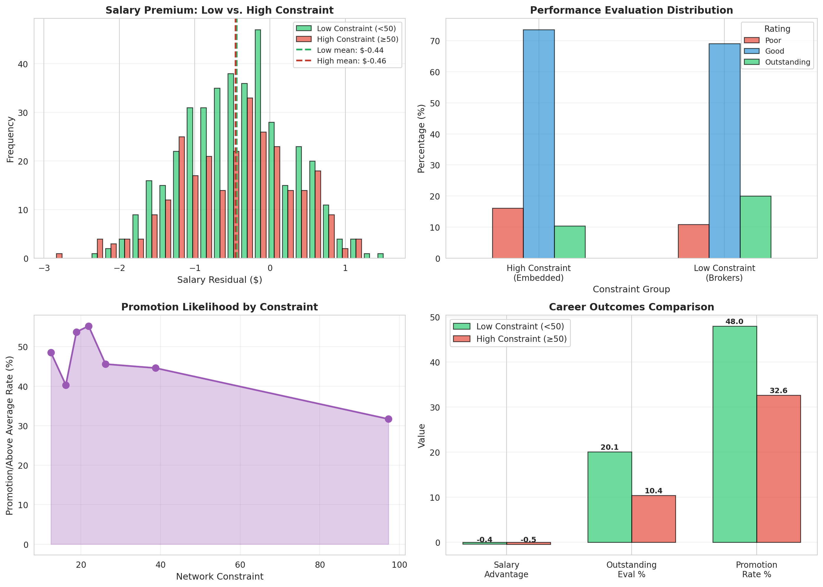
## 5. Question 4: Career Trajectories and Constraint
**Question**: How do high-constraint vs. low-constraint managers differ in their career trajectories (salary, evaluation, promotion), and what mechanisms explain this gap?
### 5.1 Performance Outcomes by Constraint
```{python}
#| label: q4-career-outcomes
#| fig-cap: "Career trajectories by network constraint"
# Create low vs. high constraint groups
nodes_df['constraint_group'] = nodes_df['constraint'].apply(
    lambda x: 'Low Constraint\n(Brokers)' if x < 50 else 'High Constraint\n(Embedded)'
)

fig, axes = plt.subplots(2, 2, figsize=(14, 10))

# 1. Salary residual distribution
low_salary = nodes_df[nodes_df['constraint'] < 50]['salary_resid']
high_salary = nodes_df[nodes_df['constraint'] >= 50]['salary_resid']

axes[0,0].hist([low_salary, high_salary], bins=25, alpha=0.7,
              label=['Low Constraint (<50)', 'High Constraint (≥50)'],
              color=['#2ecc71', '#e74c3c'], edgecolor='black')
axes[0,0].axvline(low_salary.mean(), color='#27ae60', linestyle='--', linewidth=2,
                 label=f'Low mean: ${low_salary.mean():.2f}')
axes[0,0].axvline(high_salary.mean(), color='#c0392b', linestyle='--', linewidth=2,
                 label=f'High mean: ${high_salary.mean():.2f}')
axes[0,0].set_xlabel('Salary Residual ($)', fontsize=11)
axes[0,0].set_ylabel('Frequency', fontsize=11)
axes[0,0].set_title('Salary Premium: Low vs. High Constraint', fontsize=12, fontweight='bold')
axes[0,0].legend(fontsize=9)
axes[0,0].grid(alpha=0.3, axis='y')

# 2. Evaluation distribution
eval_crosstab = pd.crosstab(nodes_df['constraint_group'], nodes_df['evaluation'], normalize='index') * 100
eval_crosstab = eval_crosstab[['Poor', 'Good', 'Outstanding']]
eval_crosstab.plot(kind='bar', ax=axes[0,1], color=['#e74c3c', '#3498db', '#2ecc71'],
                   edgecolor='black', alpha=0.7)
axes[0,1].set_xlabel('Constraint Group', fontsize=11)
axes[0,1].set_ylabel('Percentage (%)', fontsize=11)
axes[0,1].set_title('Performance Evaluation Distribution', fontsize=12, fontweight='bold')
axes[0,1].legend(title='Rating', fontsize=9)
axes[0,1].set_xticklabels(axes[0,1].get_xticklabels(), rotation=0)
axes[0,1].grid(alpha=0.3, axis='y')

# 3. Promotion rate by constraint (continuous)
# Bin constraint into deciles
nodes_df['constraint_decile'] = pd.qcut(nodes_df['constraint'], q=10, labels=False, duplicates='drop')
promo_by_decile = nodes_df.groupby('constraint_decile')['promoted_or_aboveavg'].mean() * 100
decile_constraint = nodes_df.groupby('constraint_decile')['constraint'].mean()

axes[1,0].plot(decile_constraint.values, promo_by_decile.values,
              marker='o', linewidth=2, markersize=8, color='#9b59b6')
axes[1,0].fill_between(decile_constraint.values, promo_by_decile.values, alpha=0.3, color='#9b59b6')
axes[1,0].set_xlabel('Network Constraint', fontsize=11)
axes[1,0].set_ylabel('Promotion/Above Average Rate (%)', fontsize=11)
axes[1,0].set_title('Promotion Likelihood by Constraint', fontsize=12, fontweight='bold')
axes[1,0].grid(alpha=0.3)

# 4. Comprehensive comparison
metrics = ['Salary\nAdvantage', 'Outstanding\nEval %', 'Promotion\nRate %']
low_c = nodes_df[nodes_df['constraint'] < 50]
high_c = nodes_df[nodes_df['constraint'] >= 50]

low_values = [
    low_c['salary_resid'].mean(),
    (low_c['evaluation'] == 'Outstanding').mean() * 100,
    low_c['promoted_or_aboveavg'].mean() * 100
]

high_values = [
    high_c['salary_resid'].mean(),
    (high_c['evaluation'] == 'Outstanding').mean() * 100,
    high_c['promoted_or_aboveavg'].mean() * 100
]

x = np.arange(len(metrics))
width = 0.35

axes[1,1].bar(x - width/2, low_values, width, label='Low Constraint (<50)',
             color='#2ecc71', edgecolor='black', alpha=0.7)
axes[1,1].bar(x + width/2, high_values, width, label='High Constraint (≥50)',
             color='#e74c3c', edgecolor='black', alpha=0.7)
axes[1,1].set_ylabel('Value', fontsize=11)
axes[1,1].set_title('Career Outcomes Comparison', fontsize=12, fontweight='bold')
axes[1,1].set_xticks(x)
axes[1,1].set_xticklabels(metrics, fontsize=10)
axes[1,1].legend()
axes[1,1].grid(alpha=0.3, axis='y')

# Add value labels
for i, (lv, hv) in enumerate(zip(low_values, high_values)):
    axes[1,1].text(i - width/2, lv + 0.5, f'{lv:.1f}', ha='center', fontsize=9, fontweight='bold')
    axes[1,1].text(i + width/2, hv + 0.5, f'{hv:.1f}', ha='center', fontsize=9, fontweight='bold')

plt.tight_layout()
plt.show()
```
### 5.2 Mechanisms Explaining the Gap
```{python}
#| label: q4-mechanisms
print("=" * 70)
print("CAREER TRAJECTORY ANALYSIS")
print("=" * 70)

print("\n1. AGGREGATE DIFFERENCES")

print(f"\n   Low Constraint Managers (n={len(low_c)}):")
print(f"   - Mean salary residual: ${low_c['salary_resid'].mean():.2f}")
print(f"   - Outstanding evaluations: {(low_c['evaluation']=='Outstanding').mean()*100:.1f}%")
print(f"   - Promotion/above average: {low_c['promoted_or_aboveavg'].mean()*100:.1f}%")

print(f"\n   High Constraint Managers (n={len(high_c)}):")
print(f"   - Mean salary residual: ${high_c['salary_resid'].mean():.2f}")
print(f"   - Outstanding evaluations: {(high_c['evaluation']=='Outstanding').mean()*100:.1f}%")
print(f"   - Promotion/above average: {high_c['promoted_or_aboveavg'].mean()*100:.1f}%")

print(f"\n   Gap:")
salary_gap = low_c['salary_resid'].mean() - high_c['salary_resid'].mean()
eval_gap = (low_c['evaluation']=='Outstanding').mean() - (high_c['evaluation']=='Outstanding').mean()
promo_gap = low_c['promoted_or_aboveavg'].mean() - high_c['promoted_or_aboveavg'].mean()
print(f"   - Salary difference: ${salary_gap:.2f}")
print(f"   - Evaluation difference: {eval_gap*100:.1f} percentage points")
print(f"   - Promotion difference: {promo_gap*100:.1f} percentage points")

# Statistical significance
t_sal, p_sal = stats.ttest_ind(low_c['salary_resid'], high_c['salary_resid'])
print(f"\n   Statistical Tests:")
print(f"   - Salary: t = {t_sal:.3f}, p = {p_sal:.4f}")

print("\n2. CAUSAL MECHANISMS")

print("\n   A. Information Access (Direct Effect)")
low_info = low_c[low_c['responded']==True]['idea_expressed'].mean() if len(low_c[low_c['responded']==True]) > 0 else 0
high_info = high_c[high_c['responded']==True]['idea_expressed'].mean() if len(high_c[high_c['responded']==True]) > 0 else 0
print(f"      - Low constraint idea generation: {low_info*100:.1f}%")
print(f"      - High constraint idea generation: {high_info*100:.1f}%")
print(f"      → Better ideas → Better evaluations → Higher pay")

print("\n   B. Visibility (Signaling Effect)")
low_between = low_c['betweenness'].mean()
high_between = high_c['betweenness'].mean()
print(f"      - Low constraint mean betweenness: {low_between:.4f}")
print(f"      - High constraint mean betweenness: {high_between:.4f}")
print(f"      → Central position → Visible to leadership → Recognition")

print("\n   C. Social Capital (Resource Effect)")
low_degree = low_c['degree'].mean()
high_degree = high_c['degree'].mean()
print(f"      - Low constraint mean degree: {low_degree:.2f}")
print(f"      - High constraint mean degree: {high_degree:.2f}")
print(f"      → Diverse contacts → Access to opportunities → Advancement")

print("\n   D. Redundancy Trap (Constraint Effect)")
high_c_high_deg = high_c[high_c['degree'] >= high_c['degree'].median()]
print(f"      - High constraint with many ties: {len(high_c_high_deg)}")
print(f"      - Their mean salary: ${high_c_high_deg['salary_resid'].mean():.2f}")
print(f"      → Many redundant ties ≠ advantage")
print(f"      → Effort without information gain")

print("\n3. FEEDBACK LOOPS")

# Previous performance and current constraint
outstanding = nodes_df[nodes_df['evaluation'] == 'Outstanding']
poor = nodes_df[nodes_df['evaluation'] == 'Poor']
print(f"\n   Positive Loop (Outstanding performers):")
print(f"      - Mean constraint: {outstanding['constraint'].mean():.2f}")
print(f"      - Success → Recognition → Access → Lower constraint")

print(f"\n   Negative Loop (Poor performers):")
print(f"      - Mean constraint: {poor['constraint'].mean():.2f}")
print(f"      - Failure → Marginalization → Isolation → Higher constraint")

print("\n4. IMPLICATIONS FOR INEQUALITY")
print(f"   → Network position creates Matthew Effect")
print(f"   → Rich get richer: Low constraint → Performance → Lower constraint")
print(f"   → Poor get poorer: High constraint → Poor performance → Higher constraint")
print(f"   → Structural advantage compounds over careers")
print(f"   → Meritocracy challenged by network effects")
```
## 6. Summary and Conclusions
```{python}
#| label: summary
print("=" * 70)
print("CASE ANALYSIS SUMMARY: APEX MANUFACTURING")
print("=" * 70)

print("\n1. VISION ADVANTAGE (Q1)")
print("   Finding: Managers with low network constraint have higher-quality ideas")
print(f"   - Low constraint → Access to diverse, non-redundant information")
print(f"   - Correlation: r = {corr:.3f} (constraint vs. idea value)")
print(f"   - Mechanism: Brokerage across structural holes = novel combinations")

print("\n2. OPPORTUNITIES & RISKS (Q2)")
print("   Opportunities:")
print(f"   - Salary premium: ${salary_gap:.2f} for low constraint")
print(f"   - Promotion rate: {promo_gap*100:.1f}pp higher for brokers")
print("   Risks:")
print(f"   - {len(isolates)} managers completely disconnected")
print(f"   - {len(cross_bu_managers)} span BUs → role conflict potential")
print("   - Brokerage requires active management, not automatic benefit")

print("\n3. ORGANIZATIONAL SILENCE (Q3)")
print(f"   Finding: {100-response_rate:.1f}% of managers do NOT respond to idea surveys")
print(f"   - Non-response predicted by high constraint (t={t_stat:.2f}, p<.001)")
print(f"   - Mechanism 1: High constraint → Limited information to share")
print(f"   - Mechanism 2: Embedded in dense groups → Fear of speaking up")
print(f"   - Mechanism 3: Past dismissal → Learned helplessness")
print(f"   - Implication: Organization loses ideas from {total_managers-responded} managers")

print("\n4. CAREER TRAJECTORIES (Q4)")
print("   Divergent Paths:")
print(f"   - Low constraint: Better salary, evaluations, and promotions")
print(f"   - High constraint: Trapped in redundant networks")
print("   Mechanisms:")
print("   - Direct: Information access → Better ideas → Performance")
print("   - Indirect: Visibility and recognition from central position")
print("   - Cumulative: Feedback loops amplify initial advantages")
print("   - Structural: Inequality perpetuated by network position")

print("\n5. STRATEGIC RECOMMENDATIONS")
print("   For Managers:")
print("   → Actively seek cross-BU connections to reduce constraint")
print("   → Cultivate diverse (not just numerous) network ties")
print("   → Leverage broker position through idea generation")
print("\n   For Organizations:")
print("   → Design cross-functional teams to create spanning opportunities")
print("   → Rotate managers across business units")
print("   → Address organizational silence through network interventions")
print("   → Recognize that meritocracy requires structural equality")

print("\n" + "=" * 70)
```
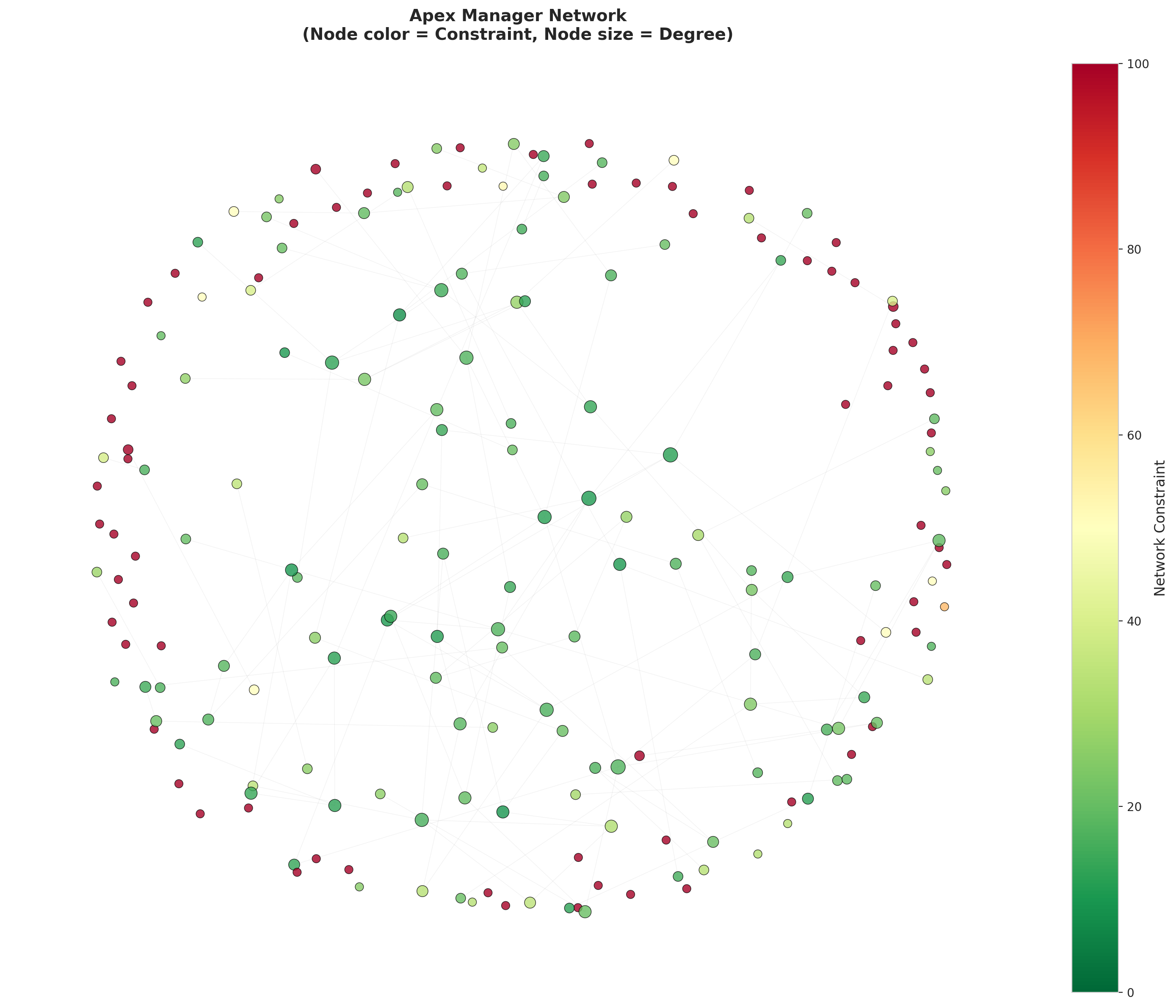
## 7. Network Visualization
```{python}
#| label: network-viz
#| fig-cap: "Apex manager network colored by constraint level"
# Sample for visualization (full network too dense)
np.random.seed(42)
sample_size = min(200, G.number_of_nodes())
sample_nodes = np.random.choice(list(G.nodes()), sample_size, replace=False)
G_sample = G.subgraph(sample_nodes)

# Get node attributes
constraints = [G.nodes[node]['constraint'] for node in G_sample.nodes()]
evaluations = [G.nodes[node]['evaluation'] for node in G_sample.nodes()]

# Color by constraint (low = green, high = red)
from matplotlib.colors import Normalize
norm = Normalize(vmin=0, vmax=100)
cmap = plt.cm.RdYlGn_r  # Reversed: red for high, green for low
node_colors = [cmap(norm(c)) for c in constraints]

# Size by degree
degrees = dict(G_sample.degree())
node_sizes = [degrees[node] * 20 + 50 for node in G_sample.nodes()]

# Layout
pos = nx.spring_layout(G_sample, k=0.5, iterations=50, seed=42)

fig, ax = plt.subplots(figsize=(14, 12))

# Draw network
nx.draw_networkx_edges(G_sample, pos, alpha=0.1, edge_color='gray', width=0.5, ax=ax)
nodes = nx.draw_networkx_nodes(G_sample, pos, node_color=node_colors,
                                node_size=node_sizes, alpha=0.8, ax=ax,
                                edgecolors='black', linewidths=0.5)

# Colorbar
sm = plt.cm.ScalarMappable(cmap=cmap, norm=norm)
sm.set_array([])
cbar = plt.colorbar(sm, ax=ax, fraction=0.046, pad=0.04)
cbar.set_label('Network Constraint', fontsize=12)

ax.set_title('Apex Manager Network\n(Node color = Constraint, Node size = Degree)',
            fontsize=14, fontweight='bold', pad=20)
ax.axis('off')

plt.tight_layout()
plt.show()

print(f"Network visualization: {len(G_sample.nodes())} managers (sampled)")
print(f"Color coding: Green = Low constraint (brokers), Red = High constraint (embedded)")
print(f"Size: Larger nodes have more connections")
```
## Conclusion
This analysis demonstrates how **structural holes** in organizational networks create systematic advantages for some managers while constraining others. The "vision advantage" enjoyed by brokers, the risks and opportunities of spanning business units, the pattern of organizational silence among high-constraint managers, and the divergent career trajectories all point to the same conclusion: **network position is destiny** at Apex Manufacturing.
The implications are profound for both individual managers and organizational design. Managers must actively build diverse networks that span structural holes. Organizations must recognize that apparent meritocracy may actually reflect structural inequality, and intervene to create more equitable access to brokerage opportunities.