Twitch Network: Exploratory Data Analysis

Week 3 - Network Analytics

Published

December 10, 2025

Introduction

This exploratory data analysis examines the Twitch network dataset, focusing on node attributes of Twitch streamers. The dataset includes information about streamer activity, content type, viewership, and affiliate status.

Code

# Load required libraries
library(tidyverse)
library(ggplot2)
library(scales)
library(knitr)

# Set theme for plots
theme_set(theme_minimal())

Code

# Read the Twitch nodes data
twitch_nodes <- read_csv("../../../data/twitch/Twitch_nodes.csv")

# Display data structure
cat("Dataset dimensions:", nrow(twitch_nodes), "rows,", ncol(twitch_nodes), "columns\n")

Dataset dimensions: 7126 rows, 6 columns

Data Overview

The Twitch dataset contains information about streamers including: - ID: Streamer identifier - Days_active: Number of days the streamer has been active - Mature_content: Whether the channel contains mature content (TRUE/FALSE) - Views: Total number of views - Affiliate: Whether the streamer has affiliate status (TRUE/FALSE) - Channel_ID: Unique channel identifier

Code

# Create a summary table of data types
data_summary <- data.frame(
  Variable = names(twitch_nodes),
  Type = sapply(twitch_nodes, class),
  Missing = sapply(twitch_nodes, function(x) sum(is.na(x))),
  Unique = sapply(twitch_nodes, function(x) length(unique(x))),
  stringsAsFactors = FALSE,
  row.names = NULL
)

kable(data_summary, caption = "Data Structure Summary", row.names = FALSE)

Data Structure Summary
Variable	Type	Unique
ID	numeric	7126
Days_active	numeric	2565
Mature_content	logical	2
Views	numeric	5822
Affiliate	logical	2
Channel_ID	numeric	7126

Distribution Analysis

Views Distribution

Code

# Calculate summary statistics
views_summary <- twitch_nodes %>%
  summarise(
    Min = min(Views),
    Q1 = quantile(Views, 0.25),
    Median = median(Views),
    Mean = mean(Views),
    Q3 = quantile(Views, 0.75),
    Max = max(Views)
  )

kable(views_summary, caption = "Views Summary Statistics", format.args = list(big.mark = ","))

Views Summary Statistics
Min	Q1	Median	Mean	Q3	Max
5	1,743	4,839.5	193,470.2	15,263	178,500,544

Code

# Create histogram with log scale
p1 <- ggplot(twitch_nodes, aes(x = Views)) +
  geom_histogram(bins = 50, fill = "#9146FF", alpha = 0.8, color = "white") +
  scale_x_log10(labels = comma) +
  geom_vline(aes(xintercept = median(Views)), 
             color = "red", linetype = "dashed", size = 1) +
  labs(title = "Distribution of Channel Views (Log Scale)",
       subtitle = paste("Median:", format(median(twitch_nodes$Views), big.mark = ",")),
       x = "Views (log scale)",
       y = "Number of Streamers") +
  theme(plot.title = element_text(hjust = 0.5, face = "bold"),
        plot.subtitle = element_text(hjust = 0.5))

p1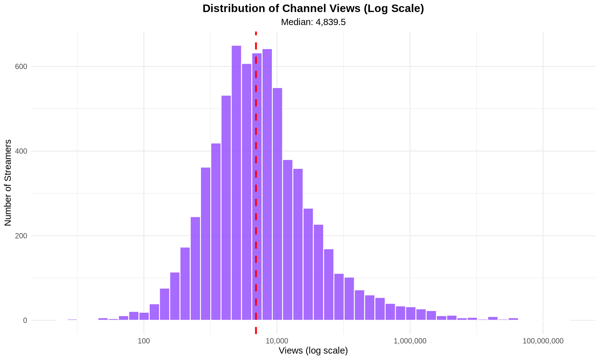

Categorical Variables

Code

# Create summary tables
categorical_summary <- bind_rows(
  twitch_nodes %>%
    count(Mature_content) %>%
    mutate(Variable = "Mature Content",
           Category = as.character(Mature_content),
           Percentage = round(n / sum(n) * 100, 1)),
  
  twitch_nodes %>%
    count(Affiliate) %>%
    mutate(Variable = "Affiliate Status",
           Category = as.character(Affiliate),
           Percentage = round(n / sum(n) * 100, 1))
) %>%
  select(Variable, Category, n, Percentage)

kable(categorical_summary, caption = "Categorical Variables Distribution")

Categorical Variables Distribution
Variable	Category	n	Percentage
Mature Content	FALSE	3238	45.4
Mature Content	TRUE	3888	54.6
Affiliate Status	FALSE	6742	94.6
Affiliate Status	TRUE	384	5.4

Relationship Analysis

Affiliate Status vs Views

Code

p2 <- twitch_nodes %>%
  mutate(Affiliate = factor(Affiliate, 
                           levels = c(FALSE, TRUE),
                           labels = c("Non-Affiliate", "Affiliate"))) %>%
  ggplot(aes(x = Affiliate, y = Views, fill = Affiliate)) +
  geom_violin(alpha = 0.6) +
  geom_boxplot(width = 0.2, alpha = 0.8) +
  scale_y_log10(labels = comma) +
  scale_fill_manual(values = c("#9146FF", "#1DB954")) +
  labs(title = "Views Distribution by Affiliate Status",
       x = "Affiliate Status",
       y = "Views (log scale)") +
  theme(legend.position = "none",
        plot.title = element_text(hjust = 0.5, face = "bold"))

p2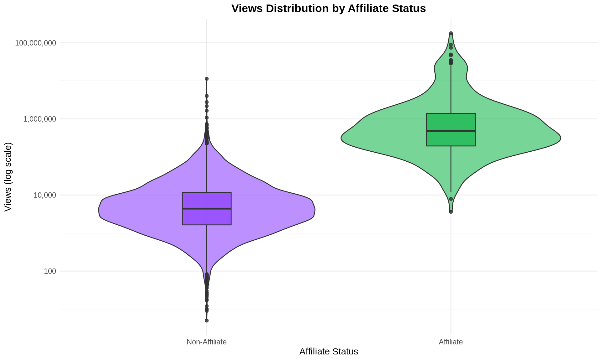

Days Active vs Views

Code

p3 <- ggplot(twitch_nodes, aes(x = Days_active, y = Views)) +
  geom_point(aes(color = Affiliate, shape = Mature_content), 
             alpha = 0.6, size = 2) +
  scale_y_log10(labels = comma) +
  scale_color_manual(values = c("#9146FF", "#1DB954"),
                     labels = c("Non-Affiliate", "Affiliate")) +
  scale_shape_manual(values = c(16, 17),
                     labels = c("Non-Mature", "Mature")) +
  geom_smooth(method = "lm", se = TRUE, alpha = 0.2) +
  labs(title = "Relationship between Days Active and Views",
       x = "Days Active",
       y = "Views (log scale)",
       color = "Affiliate Status",
       shape = "Content Type") +
  theme(plot.title = element_text(hjust = 0.5, face = "bold"))

p3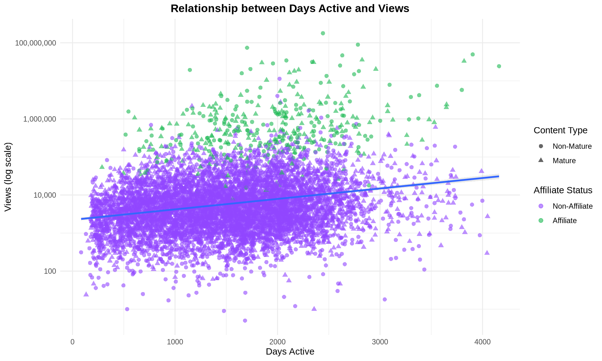

Cross-tabulation Analysis

Code

# Create detailed cross-tabulation
cross_analysis <- twitch_nodes %>%
  group_by(Mature_content, Affiliate) %>%
  summarise(
    Count = n(),
    Avg_Views = mean(Views),
    Median_Views = median(Views),
    Avg_Days_Active = mean(Days_active),
    .groups = "drop"
  ) %>%
  mutate(
    Avg_Views = round(Avg_Views),
    Avg_Days_Active = round(Avg_Days_Active),
    Mature_content = ifelse(Mature_content, "Mature", "Non-Mature"),
    Affiliate = ifelse(Affiliate, "Affiliate", "Non-Affiliate")
  )

kable(cross_analysis, 
      caption = "Average Metrics by Content Type and Affiliate Status",
      format.args = list(big.mark = ","))

Average Metrics by Content Type and Affiliate Status
Mature_content	Affiliate	Count	Avg_Views	Median_Views	Avg_Days_Active
Non-Mature	Non-Affiliate	3,041	18,934	3,261	1,487
Non-Mature	Affiliate	197	4,393,289	478,931	1,966
Mature	Non-Affiliate	3,701	17,297	5,584	1,514
Mature	Affiliate	187	2,094,097	488,224	1,913

Statistical Tests

Code

# Affiliate status comparison
affiliate_test <- t.test(log10(Views + 1) ~ Affiliate, data = twitch_nodes)
cat("T-test: Affiliate vs Non-Affiliate (log-transformed views)\n")

T-test: Affiliate vs Non-Affiliate (log-transformed views)

Code

cat("t =", round(affiliate_test$statistic, 4), "\n")

t = -54.6025

Code

cat("p-value =", format.pval(affiliate_test$p.value), "\n")

p-value = < 2.22e-16

Code

cat("Mean difference =", round(diff(affiliate_test$estimate), 4), "log units\n")

Mean difference = 2.095 log units

Top Performers

Code

# Identify top 10 channels by views
top_channels <- twitch_nodes %>%
  arrange(desc(Views)) %>%
  slice_head(n = 10) %>%
  mutate(
    Rank = row_number(),
    Views = format(Views, big.mark = ","),
    Content_Type = ifelse(Mature_content, "Mature", "Non-Mature"),
    Status = ifelse(Affiliate, "Affiliate", "Non-Affiliate")
  ) %>%
  select(Rank, Channel_ID, Views, Days_active, Content_Type, Status)

kable(top_channels, caption = "Top 10 Twitch Channels by Views")

Top 10 Twitch Channels by Views
Rank	Channel_ID	Views	Days_active	Content_Type	Status
1	27942990	178,500,544	2443	Non-Mature	Affiliate
2	20786541	89,506,813	2784	Non-Mature	Affiliate
3	56648155	74,201,622	1703	Non-Mature	Affiliate
4	261715	49,482,563	3904	Non-Mature	Affiliate
5	23735582	46,682,923	2632	Non-Mature	Affiliate
6	19623411	35,482,126	2825	Mature	Affiliate
7	39677337	34,356,681	2086	Non-Mature	Affiliate
8	497952	32,861,608	3820	Mature	Affiliate
9	30623831	31,417,100	2338	Non-Mature	Affiliate
10	30281925	30,977,250	2351	Mature	Affiliate

Key Insights

Code

# Calculate key metrics
insights <- list(
  total_streamers = nrow(twitch_nodes),
  avg_views = mean(twitch_nodes$Views),
  median_views = median(twitch_nodes$Views),
  affiliate_rate = mean(twitch_nodes$Affiliate) * 100,
  mature_content_rate = mean(twitch_nodes$Mature_content) * 100,
  views_ratio = mean(twitch_nodes$Views) / median(twitch_nodes$Views)
)

Summary of Key Findings:

Total streamers analyzed: 7,126
Highly skewed viewership: Average views (193,470) are 40x higher than median views (4,839.5), indicating extreme concentration
Affiliate rate: Only 5.4% of streamers have affiliate status
Mature content: 54.6% of channels are marked as mature
Affiliate advantage: Affiliate streamers have significantly higher viewership (p < 0.001)

This analysis provides context for understanding how node attributes might relate to network centrality measures in the Twitch streamer ecosystem.