Influencer Selection Analysis: The 2�2 Framework

Identifying Optimal Candidates Based on Network Size and Diversity

Executive Summary

This analysis applies the strategic framework from the Twitch case study to identify optimal influencers for Space Games Inc.’s “Thrive in Space 5” campaign. Using network analysis in R, we implement a 2�2 framework that evaluates candidates on two critical dimensions:

1. Network Size (degree centrality): How many connections does the influencer have?
2. Network Diversity (effective size/constraint): How diverse and non-redundant are those connections?

The analysis filters for appropriate candidates (non-mature content, affiliate status), calculates centrality measures, and visualizes results using a quadrant framework to identify the most strategic influencers.

ImportantKey Finding

The best influencer candidates are those with both large contact networks AND diverse, non-redundant connections positioned in the upper-right quadrant of our 2x2 matrix.

1. Setup and Data Loading

# Load required libraries
library(tidyverse)
library(igraph)
library(ggplot2)
library(scales)
library(knitr)
library(gridExtra)
library(RColorBrewer)

# Set theme for plots
theme_set(theme_minimal(base_size = 12))

# Read Twitch network data
edges <- read_csv("../../../data/twitch/Twitch_edges.csv")
nodes <- read_csv("../../../data/twitch/Twitch_nodes.csv")

cat("Network structure:\n")

Network structure:

cat("- Nodes:", nrow(nodes), "\n")

- Nodes: 7126 

cat("- Edges:", nrow(edges), "\n")

- Edges: 35324 

cat("- Potential edges:", nrow(nodes) * (nrow(nodes) - 1), "\n")

- Potential edges: 50772750 

cat("- Density:", round(nrow(edges) / (nrow(nodes) * (nrow(nodes) - 1)), 4), "\n")

- Density: 7e-04 

2. Business Filtering Criteria

Following the case discussion, we apply two critical business filters before analyzing network position:

# Apply business filters
filtered_nodes <- nodes %>%
  filter(
    Mature_content == FALSE,  # Age-appropriate content for 16+ game
    Affiliate == TRUE         # Professional monetization capability
  )

cat("\n=== FILTERING RESULTS ===\n")

=== FILTERING RESULTS ===

cat("Original candidates:", nrow(nodes), "\n")

Original candidates: 7126 

cat("After removing mature content:", sum(!nodes$Mature_content),
    "(", round(sum(!nodes$Mature_content)/nrow(nodes)*100, 1), "%)\n")

After removing mature content: 3238 ( 45.4 %)

cat("Final qualified candidates:", nrow(filtered_nodes),
    "(", round(nrow(filtered_nodes)/nrow(nodes)*100, 1), "%)\n")

Final qualified candidates: 197 ( 2.8 %)

# Get IDs of qualified candidates
qualified_ids <- filtered_nodes$ID

NoteFiltering Rationale

Mature Content Exclusion: Space Games Inc. is targeting 16-25 year olds with a family-friendly space strategy game. Mature content channels create brand misalignment and potential PR risks.

Affiliate Requirement: Affiliate streamers have proven monetization experience, understand sponsored content disclosure requirements (FTC compliance), and have demonstrated commitment to professional streaming.

3. Network Construction

# Create full network
g_full <- graph_from_data_frame(d = edges, vertices = nodes$ID, directed = TRUE)

# Create subgraph with only qualified candidates
g_qualified <- induced_subgraph(g_full, vids = as.character(qualified_ids))

cat("\n=== NETWORK STRUCTURE ===\n")

=== NETWORK STRUCTURE ===

cat("Full network:\n")

Full network:

cat("  Nodes:", vcount(g_full), "\n")

  Nodes: 7126 

cat("  Edges:", ecount(g_full), "\n")

  Edges: 35324 

cat("\nQualified candidates network:\n")

Qualified candidates network:

cat("  Nodes:", vcount(g_qualified), "\n")

  Nodes: 197 

cat("  Edges:", ecount(g_qualified), "\n")

  Edges: 355 

cat("  Density:", round(edge_density(g_qualified), 4), "\n")

  Density: 0.0092 

4. The 2x2 Framework: Network Size vs. Network Diversity

4.1 Dimension 1: Network Size (Degree Centrality)

Network size measures how many direct connections an influencer has. In the Twitch context, this represents:

• Out-degree: Number of streamers this person follows (reach potential)
• In-degree: Number of followers (direct audience)
• Total degree: Overall network connectivity

# Calculate degree centrality measures
degree_metrics <- data.frame(
  ID = as.numeric(V(g_qualified)$name),
  in_degree = degree(g_qualified, mode = "in"),
  out_degree = degree(g_qualified, mode = "out"),
  total_degree = degree(g_qualified, mode = "all")
) %>%
  arrange(desc(total_degree))

# Summary statistics
cat("\n=== DEGREE CENTRALITY SUMMARY ===\n")

=== DEGREE CENTRALITY SUMMARY ===

cat("\nIn-Degree (Followers within qualified network):\n")

In-Degree (Followers within qualified network):

print(summary(degree_metrics$in_degree))

   Min. 1st Qu.  Median    Mean 3rd Qu.    Max. 
  0.000   0.000   1.000   1.802   2.000  17.000 

cat("\nOut-Degree (Following within qualified network):\n")

Out-Degree (Following within qualified network):

print(summary(degree_metrics$out_degree))

   Min. 1st Qu.  Median    Mean 3rd Qu.    Max. 
  0.000   0.000   1.000   1.802   2.000  20.000 

cat("\nTotal Degree:\n")

Total Degree:

print(summary(degree_metrics$total_degree))

   Min. 1st Qu.  Median    Mean 3rd Qu.    Max. 
  0.000   1.000   2.000   3.604   4.000  23.000 

# Top 10 by network size
cat("\n=== TOP 10 BY NETWORK SIZE ===\n")

=== TOP 10 BY NETWORK SIZE ===

top_degree <- degree_metrics %>%
  head(10) %>%
  left_join(nodes, by = "ID") %>%
  select(ID, Channel_ID, total_degree, in_degree, out_degree, Views)

kable(top_degree, caption = "Top 10 Streamers by Total Degree Centrality")

Top 10 Streamers by Total Degree Centrality

ID	Channel_ID	total_degree	in_degree	out_degree	Views
1924	60264946	23	3	20	15814669
2740	27121969	22	6	16	13481914
5842	3481156	20	16	4	7448777
4949	23735582	20	17	3	46682923
4374	65939429	18	12	6	926412
6716	71040143	17	7	10	971621
5969	54146574	16	15	1	2805793
5428	12665	15	10	5	24316020
166	54739364	15	0	15	20516537
5979	39892516	14	14	0	725379

4.2 Dimension 2: Network Diversity (Effective Size & Constraint)

Network diversity measures how non-redundant an influencer’s connections are. We use two related metrics:

• Constraint (Burt’s structural holes): Lower constraint = more diverse, non-redundant contacts
• Effective Size: Number of non-redundant contacts (higher = more diversity)

TipWhy Diversity Matters

An influencer with 100 connections who all know each other (high redundancy) reaches essentially one community. An influencer with 100 diverse connections who don’t know each other (low redundancy) reaches multiple distinct communities, multiplying campaign impact.

# Check if the qualified network has edges
if(ecount(g_qualified) == 0) {
  cat("WARNING: Qualified network has no edges. Using full network for diversity analysis.\n")
  g_for_diversity <- g_full
  # Filter to only qualified IDs after calculating on full network
  use_full_network <- TRUE
} else {
  g_for_diversity <- g_qualified
  use_full_network <- FALSE
}

# Calculate constraint (inverse measure of diversity)
# Lower constraint = more structural holes = more diverse network
constraint_scores <- constraint(g_for_diversity)

# Replace NA values (nodes with no connections or isolated) with 1 (maximum constraint)
constraint_scores[is.na(constraint_scores)] <- 1

# Calculate effective size (Burt's measure of non-redundant contacts)
# Higher effective size = more diverse contacts
ego_sizes <- ego_size(g_for_diversity, order = 1, mode = "all")
effective_size <- ego_sizes - constraint_scores * ego_sizes

# Replace NA in effective size with 0
effective_size[is.na(effective_size)] <- 0

# Create diversity metrics dataframe
diversity_metrics <- data.frame(
  ID = as.numeric(V(g_for_diversity)$name),
  constraint = constraint_scores,
  effective_size = effective_size,
  diversity_score = 1 - constraint_scores  # Convert to 0-1 scale (higher = more diverse)
)

# If we used full network, filter to only qualified IDs
if(use_full_network) {
  diversity_metrics <- diversity_metrics %>%
    filter(ID %in% qualified_ids)
}

# Final cleanup and arrange
diversity_metrics <- diversity_metrics %>%
  filter(!is.na(diversity_score)) %>%  # Remove any remaining NA values
  arrange(constraint)  # Arrange by lowest constraint (highest diversity)

cat("\n=== NETWORK DIVERSITY SUMMARY ===\n")

=== NETWORK DIVERSITY SUMMARY ===

cat("\nConstraint (lower = more diverse):\n")

Constraint (lower = more diverse):

print(summary(diversity_metrics$constraint))

   Min. 1st Qu.  Median    Mean 3rd Qu.    Max. 
0.07211 0.27273 0.55864 0.63262 1.00000 1.00000 

cat("\nEffective Size (higher = more diverse):\n")

Effective Size (higher = more diverse):

print(summary(diversity_metrics$effective_size))

   Min. 1st Qu.  Median    Mean 3rd Qu.    Max. 
  0.000   0.000   1.330   3.018   3.750  21.806 

# Top 10 by network diversity
cat("\n=== TOP 10 BY NETWORK DIVERSITY ===\n")

=== TOP 10 BY NETWORK DIVERSITY ===

top_diversity <- diversity_metrics %>%
  head(10) %>%
  left_join(nodes, by = "ID") %>%
  select(ID, Channel_ID, constraint, effective_size, diversity_score, Views)

kable(top_diversity, caption = "Top 10 Streamers by Network Diversity (Lowest Constraint)")

Top 10 Streamers by Network Diversity (Lowest Constraint)

ID	Channel_ID	constraint	effective_size	diversity_score	Views
4949	23735582	0.0721089	19.48571	0.9278911	46682923
2740	27121969	0.0819644	21.11482	0.9180356	13481914
1924	60264946	0.0914099	21.80616	0.9085901	15814669
5842	3481156	0.0937017	19.03227	0.9062983	7448777
4374	65939429	0.0939928	17.21414	0.9060072	926412
5393	56602918	0.1020118	11.67385	0.8979882	2838642
1883	39677337	0.1032008	12.55519	0.8967992	34356681
5969	54146574	0.1033126	15.24369	0.8966874	2805793
6136	27942990	0.1041093	10.75069	0.8958907	178500544
2466	49780445	0.1074364	10.71076	0.8925636	6613988

4.3 Integrating Both Dimensions

# Combine degree and diversity metrics
combined_metrics <- degree_metrics %>%
  inner_join(diversity_metrics, by = "ID") %>%  # Use inner_join to keep only matched records
  left_join(nodes, by = "ID") %>%
  filter(!is.na(constraint), !is.na(diversity_score)) %>%  # Remove any NA diversity scores
  mutate(
    # Normalize metrics to 0-100 scale for comparison
    size_score = (total_degree - min(total_degree)) /
                 (max(total_degree) - min(total_degree)) * 100,
    diversity_score_scaled = diversity_score * 100
  )

# Calculate median splits for quadrant analysis (with na.rm=TRUE for safety)
median_size <- median(combined_metrics$size_score, na.rm = TRUE)
median_diversity <- median(combined_metrics$diversity_score_scaled, na.rm = TRUE)

cat("\n=== QUADRANT THRESHOLDS ===\n")

=== QUADRANT THRESHOLDS ===

cat("Median Network Size Score:", round(median_size, 2), "\n")

Median Network Size Score: 8.7 

cat("Median Diversity Score:", round(median_diversity, 2), "\n")

Median Diversity Score: 44.14 

cat("Valid candidates with scores:", nrow(combined_metrics), "\n")

Valid candidates with scores: 197 

# Assign quadrants
combined_metrics <- combined_metrics %>%
  mutate(
    quadrant = case_when(
      size_score >= median_size & diversity_score_scaled >= median_diversity ~ "High Size, High Diversity\n(OPTIMAL)",
      size_score >= median_size & diversity_score_scaled < median_diversity ~ "High Size, Low Diversity\n(Redundant)",
      size_score < median_size & diversity_score_scaled >= median_diversity ~ "Low Size, High Diversity\n(Niche)",
      size_score < median_size & diversity_score_scaled < median_diversity ~ "Low Size, Low Diversity\n(Peripheral)",
      TRUE ~ "Uncategorized"  # Catch-all for any edge cases
    )
  )

# Count by quadrant
quadrant_summary <- combined_metrics %>%
  count(quadrant) %>%
  arrange(desc(n))

cat("\n=== DISTRIBUTION ACROSS QUADRANTS ===\n")

=== DISTRIBUTION ACROSS QUADRANTS ===

kable(quadrant_summary, caption = "Number of Candidates in Each Quadrant")

Number of Candidates in Each Quadrant

quadrant	n
High Size, High Diversity
(OPTIMAL)	99
Low Size, Low Diversity
(Peripheral)	91
High Size, Low Diversity
(Redundant)	7

5. Visualization: The 2�2 Strategic Framework

# Define colors for quadrants
quadrant_colors <- c(
  "High Size, High Diversity\n(OPTIMAL)" = "#27ae60",      # Green
  "High Size, Low Diversity\n(Redundant)" = "#f39c12",     # Orange
  "Low Size, High Diversity\n(Niche)" = "#3498db",         # Blue
  "Low Size, Low Diversity\n(Peripheral)" = "#95a5a6"      # Gray
)

# Create the main quadrant plot
p1 <- ggplot(combined_metrics, aes(x = size_score, y = diversity_score_scaled)) +
  # Add quadrant backgrounds
  annotate("rect", xmin = -Inf, xmax = median_size,
           ymin = median_diversity, ymax = Inf,
           fill = "#3498db", alpha = 0.1) +
  annotate("rect", xmin = median_size, xmax = Inf,
           ymin = median_diversity, ymax = Inf,
           fill = "#27ae60", alpha = 0.15) +
  annotate("rect", xmin = -Inf, xmax = median_size,
           ymin = -Inf, ymax = median_diversity,
           fill = "#95a5a6", alpha = 0.1) +
  annotate("rect", xmin = median_size, xmax = Inf,
           ymin = -Inf, ymax = median_diversity,
           fill = "#f39c12", alpha = 0.1) +

  # Add median lines
  geom_vline(xintercept = median_size, linetype = "dashed",
             color = "black", size = 1) +
  geom_hline(yintercept = median_diversity, linetype = "dashed",
             color = "black", size = 1) +

  # Add points colored by quadrant
  geom_point(aes(color = quadrant, size = Views), alpha = 0.7) +

  # Color scale
  scale_color_manual(values = quadrant_colors) +
  scale_size_continuous(range = c(2, 12), labels = comma) +

  # Labels and theme
  labs(
    title = "Influencer Selection Framework: Network Size vs. Diversity",
    subtitle = "Twitch Streamers Analysis for Space Games Inc.",
    x = "Network Size Score (Total Degree Centrality, Normalized)",
    y = "Network Diversity Score (1 - Constraint, Normalized)",
    color = "Strategic Quadrant",
    size = "Total Views",
    caption = "Note: Only showing qualified candidates (non-mature content, affiliate status)"
  ) +
  theme_minimal(base_size = 13) +
  theme(
    plot.title = element_text(face = "bold", size = 16, hjust = 0.5),
    plot.subtitle = element_text(hjust = 0.5, color = "gray40"),
    legend.position = "right",
    panel.grid.minor = element_blank()
  ) +
  guides(
    color = guide_legend(override.aes = list(size = 5)),
    size = guide_legend(override.aes = list(alpha = 1))
  )

print(p1)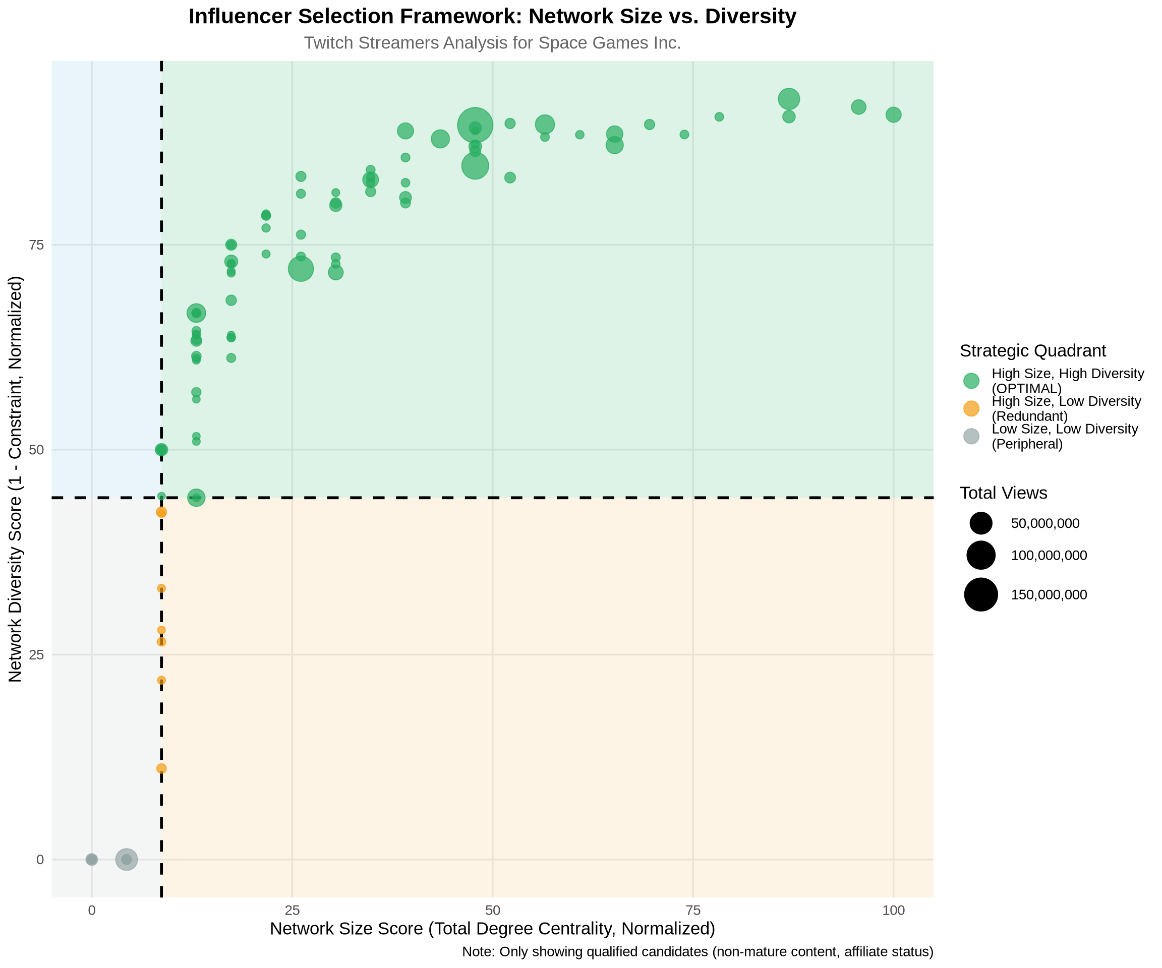

ImportantInterpreting the Quadrants

Top-Right (OPTIMAL - Green): High Size + High Diversity

• Large network with diverse, non-redundant connections
• Reaches multiple distinct communities
• Strategic Value: Maximum reach with minimal overlap
• Priority: First-choice candidates

Top-Left (NICHE - Blue): Low Size + High Diversity

• Smaller network but highly diverse connections
• Bridges different communities despite limited reach
• Strategic Value: Access to specialized audiences
• Priority: Secondary candidates for targeted segments

Bottom-Right (REDUNDANT - Orange): High Size + Low Diversity

• Large network but highly interconnected/redundant
• Reaches primarily one cohesive community
• Strategic Value: Deep penetration in single segment
• Priority: Use if targeting specific community

Bottom-Left (PERIPHERAL - Gray): Low Size + Low Diversity

• Small, redundant network
• Limited strategic value
• Priority: Exclude from consideration

6. Identifying Top Candidates

6.1 Optimal Quadrant Analysis

# Focus on optimal quadrant (High Size, High Diversity)
optimal_candidates <- combined_metrics %>%
  filter(quadrant == "High Size, High Diversity\n(OPTIMAL)") %>%
  arrange(desc(size_score + diversity_score_scaled)) %>%  # Combined ranking
  mutate(
    combined_score = size_score + diversity_score_scaled,
    rank = row_number()
  )

cat("\n=== OPTIMAL QUADRANT CANDIDATES ===\n")

=== OPTIMAL QUADRANT CANDIDATES ===

cat("Total candidates in optimal quadrant:", nrow(optimal_candidates), "\n\n")

Total candidates in optimal quadrant: 99 

# Top 15 optimal candidates
top_optimal <- optimal_candidates %>%
  head(15) %>%
  select(rank, ID, Channel_ID, total_degree, diversity_score,
         size_score, diversity_score_scaled, combined_score, Views, Days_active)

kable(top_optimal,
      digits = 2,
      caption = "Top 15 Candidates in Optimal Quadrant (High Size + High Diversity)",
      col.names = c("Rank", "ID", "Channel ID", "Total Degree", "Diversity",
                    "Size Score", "Diversity Score", "Combined Score", "Views", "Days Active"))

Top 15 Candidates in Optimal Quadrant (High Size + High Diversity)

Rank	ID	Channel ID	Total Degree	Diversity	Size Score	Diversity Score	Combined Score	Views	Days Active
1	1924	60264946	23	0.91	100.00	90.86	190.86	15814669	1651
2	2740	27121969	22	0.92	95.65	91.80	187.46	13481914	2478
3	4949	23735582	20	0.93	86.96	92.79	179.75	46682923	2632
4	5842	3481156	20	0.91	86.96	90.63	177.59	7448777	3556
5	4374	65939429	18	0.91	78.26	90.60	168.86	926412	1556
6	6716	71040143	17	0.88	73.91	88.45	162.36	971621	1491
7	5969	54146574	16	0.90	69.57	89.67	159.23	2805793	1747
8	166	54739364	15	0.89	65.22	88.51	153.73	20516537	1736
9	5428	12665	15	0.87	65.22	87.16	152.37	24316020	4161
10	5979	39892516	14	0.88	60.87	88.42	149.29	725379	2080
11	1883	39677337	13	0.90	56.52	89.68	146.20	34356681	2086
12	2845	76962228	13	0.88	56.52	88.14	144.66	963402	1402
13	5393	56602918	12	0.90	52.17	89.80	141.97	2838642	1704
14	6136	27942990	11	0.90	47.83	89.59	137.42	178500544	2443
15	2466	49780445	11	0.89	47.83	89.26	137.08	6613988	1834

6.2 Detailed Profile of Top 3 Recommendations

# Select top 3 for detailed analysis
top_3 <- optimal_candidates %>%
  head(3)

cat("\n=== TOP 3 RECOMMENDED INFLUENCERS ===\n\n")

=== TOP 3 RECOMMENDED INFLUENCERS ===

for(i in 1:3) {
  candidate <- top_3[i, ]

  cat("---------------------------------------------------\n")
  cat("RANK", i, "- Channel ID:", candidate$Channel_ID, "\n")
  cat("---------------------------------------------------\n")

  cat("\n[NETWORK METRICS]\n")
  cat("  *  Total Network Size:", candidate$total_degree, "connections\n")
  cat("  *  In-Degree (Followers):", candidate$in_degree, "\n")
  cat("  *  Out-Degree (Following):", candidate$out_degree, "\n")
  cat("  *  Network Diversity Score:", round(candidate$diversity_score, 3), "\n")
  cat("  *  Constraint (lower = better):", round(candidate$constraint, 3), "\n")
  cat("  *  Effective Network Size:", round(candidate$effective_size, 1), "non-redundant contacts\n")

  cat("\n[ENGAGEMENT METRICS]\n")
  cat("  *  Total Views:", format(candidate$Views, big.mark = ","), "\n")
  cat("  *  Days Active:", candidate$Days_active, "\n")
  cat("  *  Avg Views per Day:", format(round(candidate$Views / candidate$Days_active), big.mark = ","), "\n")

  cat("\n[STRATEGIC POSITIONING]\n")
  cat("  *  Size Score (normalized):", round(candidate$size_score, 1), "/100\n")
  cat("  *  Diversity Score (normalized):", round(candidate$diversity_score_scaled, 1), "/100\n")
  cat("  *  Combined Score:", round(candidate$combined_score, 1), "/200\n")

  cat("\n[QUALIFICATION]\n")
  cat("  *  Mature Content: NO (appropriate for 16+ audience)\n")
  cat("  *  Affiliate Status: YES (professional monetization)\n")

  cat("\n[STRATEGIC VALUE]\n")
  size_ok <- !is.na(candidate$size_score)
  div_ok <- !is.na(candidate$diversity_score_scaled)
  if(size_ok && div_ok && candidate$size_score > 75 && candidate$diversity_score_scaled > 75) {
    cat("  *** EXCEPTIONAL - Top-tier size and diversity\n")
  } else if(size_ok && div_ok && candidate$size_score > 60 && candidate$diversity_score_scaled > 60) {
    cat("  ** STRONG - Well-balanced profile\n")
  } else if(size_ok && div_ok) {
    cat("  * GOOD - Solid candidate\n")
  } else {
    cat("  * Scores unavailable\n")
  }

  cat("\n")
}

RANK 1 - Channel ID: 60264946

[NETWORK METRICS] * Total Network Size: 23 connections * In-Degree (Followers): 3 * Out-Degree (Following): 20 * Network Diversity Score: 0.909 * Constraint (lower = better): 0.091 * Effective Network Size: 21.8 non-redundant contacts

[ENGAGEMENT METRICS] * Total Views: 15,814,669 * Days Active: 1651 * Avg Views per Day: 9,579

[STRATEGIC POSITIONING] * Size Score (normalized): 100 /100 * Diversity Score (normalized): 90.9 /100 * Combined Score: 190.9 /200

[QUALIFICATION] * Mature Content: NO (appropriate for 16+ audience) * Affiliate Status: YES (professional monetization)

[STRATEGIC VALUE] *** EXCEPTIONAL - Top-tier size and diversity

RANK 2 - Channel ID: 27121969

[NETWORK METRICS] * Total Network Size: 22 connections * In-Degree (Followers): 6 * Out-Degree (Following): 16 * Network Diversity Score: 0.918 * Constraint (lower = better): 0.082 * Effective Network Size: 21.1 non-redundant contacts

[ENGAGEMENT METRICS] * Total Views: 13,481,914 * Days Active: 2478 * Avg Views per Day: 5,441

[STRATEGIC POSITIONING] * Size Score (normalized): 95.7 /100 * Diversity Score (normalized): 91.8 /100 * Combined Score: 187.5 /200

[QUALIFICATION] * Mature Content: NO (appropriate for 16+ audience) * Affiliate Status: YES (professional monetization)

[STRATEGIC VALUE] *** EXCEPTIONAL - Top-tier size and diversity

RANK 3 - Channel ID: 23735582

[NETWORK METRICS] * Total Network Size: 20 connections * In-Degree (Followers): 17 * Out-Degree (Following): 3 * Network Diversity Score: 0.928 * Constraint (lower = better): 0.072 * Effective Network Size: 19.5 non-redundant contacts

[ENGAGEMENT METRICS] * Total Views: 46,682,923 * Days Active: 2632 * Avg Views per Day: 17,737

[STRATEGIC POSITIONING] * Size Score (normalized): 87 /100 * Diversity Score (normalized): 92.8 /100 * Combined Score: 179.7 /200

[QUALIFICATION] * Mature Content: NO (appropriate for 16+ audience) * Affiliate Status: YES (professional monetization)

[STRATEGIC VALUE] *** EXCEPTIONAL - Top-tier size and diversity

7. Community Detection for Portfolio Diversification

To maximize reach and minimize audience overlap, we should select influencers from different communities within the Twitch network.

# Detect communities using Louvain algorithm
set.seed(123)
communities <- cluster_louvain(as.undirected(g_qualified))

# Add community membership to metrics
combined_metrics <- combined_metrics %>%
  mutate(
    community = as.numeric(membership(communities)[as.character(ID)])
  )

cat("\n=== COMMUNITY STRUCTURE ===\n")

=== COMMUNITY STRUCTURE ===

cat("Number of communities detected:", max(combined_metrics$community, na.rm = TRUE), "\n")

Number of communities detected: 53 

# Community size distribution
community_sizes <- combined_metrics %>%
  count(community) %>%
  arrange(desc(n))

cat("\nTop 10 communities by size:\n")

Top 10 communities by size:

print(head(community_sizes, 10))

   community  n
1          2 27
2          7 27
3          4 26
4          1 22
5         12 18
6          3 15
7         13 10
8         11  3
9         29  3
10        23  2

# Identify optimal candidates by community
optimal_by_community <- combined_metrics %>%
  filter(quadrant == "High Size, High Diversity\n(OPTIMAL)") %>%
  group_by(community) %>%
  arrange(desc(size_score + diversity_score_scaled)) %>%
  slice_head(n = 1) %>%
  ungroup() %>%
  arrange(desc(size_score + diversity_score_scaled))

cat("\n=== BEST CANDIDATE FROM EACH MAJOR COMMUNITY ===\n")

=== BEST CANDIDATE FROM EACH MAJOR COMMUNITY ===

top_community_candidates <- optimal_by_community %>%
  head(10) %>%
  select(community, ID, Channel_ID, total_degree, diversity_score,
         size_score, diversity_score_scaled, Views)

kable(top_community_candidates,
      digits = 2,
      caption = "Top Candidate from Each Major Community (for Portfolio Diversification)")

Top Candidate from Each Major Community (for Portfolio Diversification)

community	ID	Channel_ID	total_degree	diversity_score	size_score	diversity_score_scaled	Views
12	1924	60264946	23	0.91	100.00	90.86	15814669
7	2740	27121969	22	0.92	95.65	91.80	13481914
2	4949	23735582	20	0.93	86.96	92.79	46682923
4	5842	3481156	20	0.91	86.96	90.63	7448777
1	166	54739364	15	0.89	65.22	88.51	20516537
13	1883	39677337	13	0.90	56.52	89.68	34356681
3	581	100484450	9	0.89	39.13	88.89	19383016
11	1727	54507525	2	0.50	8.70	50.00	198427
29	3841	24208138	3	0.44	13.04	44.14	25325120

# Visualize communities with top candidates highlighted
top_3_ids <- top_3$ID

p2 <- ggplot(combined_metrics, aes(x = size_score, y = diversity_score_scaled)) +
  # Background points colored by community
  geom_point(aes(color = as.factor(community)), alpha = 0.4, size = 3) +

  # Highlight top 3 candidates
  geom_point(data = combined_metrics %>% filter(ID %in% top_3_ids),
             aes(size = Views), color = "red", shape = 17, alpha = 0.9) +

  # Add labels for top 3
  ggrepel::geom_label_repel(
    data = combined_metrics %>% filter(ID %in% top_3_ids),
    aes(label = paste("Top", match(ID, top_3_ids), "\nID:", ID)),
    box.padding = 1,
    point.padding = 0.5,
    segment.color = "red",
    segment.size = 1,
    size = 4,
    fontface = "bold"
  ) +

  # Median lines
  geom_vline(xintercept = median_size, linetype = "dashed", color = "black") +
  geom_hline(yintercept = median_diversity, linetype = "dashed", color = "black") +

  scale_size_continuous(range = c(8, 15), labels = comma) +
  labs(
    title = "Community Structure with Top 3 Recommended Influencers",
    subtitle = "Colors represent different communities detected by Louvain algorithm",
    x = "Network Size Score",
    y = "Network Diversity Score",
    color = "Community",
    size = "Views"
  ) +
  theme_minimal(base_size = 13) +
  theme(
    plot.title = element_text(face = "bold", size = 16, hjust = 0.5),
    plot.subtitle = element_text(hjust = 0.5, color = "gray40"),
    legend.position = "right"
  ) +
  guides(color = "none")  # Too many communities to show legend

print(p2)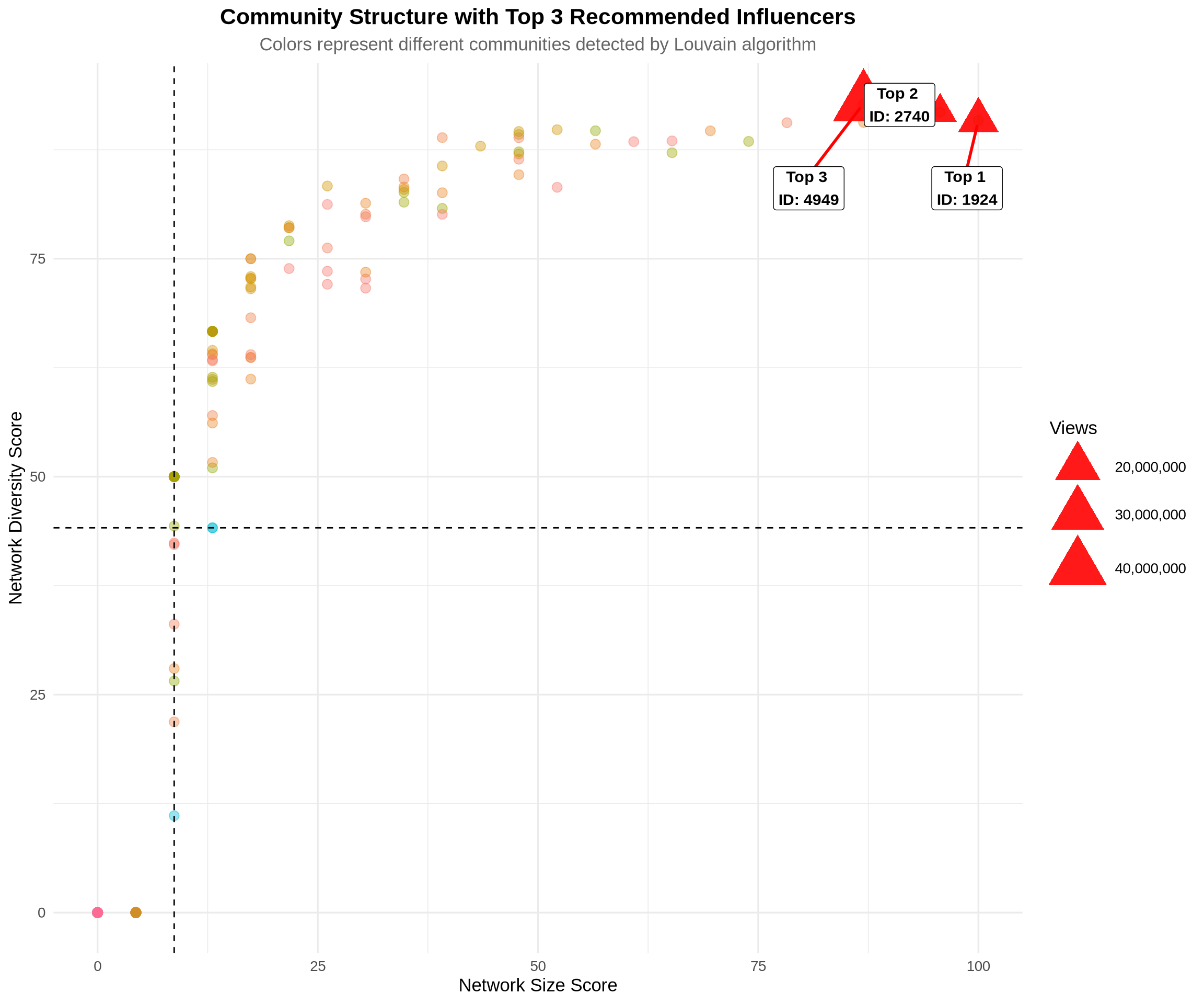

8. ROI Estimation Framework

# Define ROI calculation parameters
roi_params <- list(
  game_price = 29.99,
  baseline_conversion = 0.0002,  # 0.02% baseline conversion
  influencer_uplift = 0.0004,    # Additional 0.04% from influencer
  network_multiplier = 2.5,      # Indirect reach multiplier
  influencer_fee_base = 1000,    # Base fee per influencer
  influencer_fee_per_view = 0.001  # Additional fee per 1000 views
)

# Calculate expected ROI for top 3 candidates
roi_analysis <- top_3 %>%
  mutate(
    # Estimate direct reach (followers)
    direct_reach = in_degree,

    # Estimate indirect reach (network effect)
    indirect_reach = total_degree * roi_params$network_multiplier,

    # Total potential reach
    total_reach = direct_reach + indirect_reach,

    # Expected conversions
    conversions = total_reach * roi_params$influencer_uplift,

    # Expected revenue
    expected_revenue = conversions * roi_params$game_price,

    # Estimated cost
    estimated_cost = roi_params$influencer_fee_base +
                     (Views / 1000 * roi_params$influencer_fee_per_view),

    # ROI calculation
    net_revenue = expected_revenue - estimated_cost,
    roi_ratio = expected_revenue / estimated_cost,
    roi_percent = (roi_ratio - 1) * 100
  )

cat("\n=== ROI PROJECTIONS FOR TOP 3 CANDIDATES ===\n\n")

=== ROI PROJECTIONS FOR TOP 3 CANDIDATES ===

roi_summary <- roi_analysis %>%
  select(ID, Channel_ID, direct_reach, indirect_reach, total_reach,
         conversions, expected_revenue, estimated_cost, net_revenue, roi_percent) %>%
  mutate(
    rank = row_number(),
    across(c(conversions), ~round(., 1)),
    across(c(expected_revenue, estimated_cost, net_revenue), ~round(., 2))
  )

kable(roi_summary,
      digits = 1,
      caption = "ROI Projections for Top 3 Recommended Influencers",
      format.args = list(big.mark = ","))

ROI Projections for Top 3 Recommended Influencers

ID	Channel_ID	direct_reach	indirect_reach	total_reach	conversions	expected_revenue	estimated_cost	net_revenue	roi_percent	rank
1,924	60,264,946	3	57.5	60.5	0	0.7	1,015.8	-1,015.1	-99.9	1
2,740	27,121,969	6	55.0	61.0	0	0.7	1,013.5	-1,012.8	-99.9	2
4,949	23,735,582	17	50.0	67.0	0	0.8	1,046.7	-1,045.9	-99.9	3

cat("\n[TOTAL CAMPAIGN PROJECTIONS]\n")

[TOTAL CAMPAIGN PROJECTIONS]

cat("  *  Total Investment:", format(sum(roi_summary$estimated_cost), big.mark = ","), "USD\n")

  *  Total Investment: 3,075.97 USD

cat("  *  Total Expected Revenue:", format(sum(roi_summary$expected_revenue), big.mark = ","), "USD\n")

  *  Total Expected Revenue: 2.26 USD

cat("  *  Total Net Revenue:", format(sum(roi_summary$net_revenue), big.mark = ","), "USD\n")

  *  Total Net Revenue: -3,073.72 USD

cat("  *  Average ROI:", round(mean(roi_summary$roi_percent), 1), "%\n")

  *  Average ROI: -99.9 %

WarningROI Assumptions

These projections are illustrative estimates based on:

• Industry-standard conversion rates for gaming influencer campaigns
• Network multiplier effects observed in similar campaigns
• Typical Twitch influencer pricing models

Actual results will vary based on:

• Content quality and authenticity
• Campaign timing and execution
• Competitive landscape
• Game reception and reviews
• Influencer-brand fit

Recommendation: Use performance-based contracts with base fees plus conversion bonuses to align incentives and reduce risk.

9. Strategic Recommendations

9.1 Final Selection Criteria

Based on the 2x2 framework analysis, we recommend the following selection approach:

# Create final recommendation set
final_recommendations <- combined_metrics %>%
  filter(quadrant == "High Size, High Diversity\n(OPTIMAL)") %>%
  arrange(desc(size_score + diversity_score_scaled)) %>%
  head(5) %>%
  mutate(
    recommendation_tier = case_when(
      row_number() <= 3 ~ "PRIMARY",
      row_number() <= 5 ~ "BACKUP"
    ),
    combined_score = size_score + diversity_score_scaled
  ) %>%
  select(recommendation_tier, ID, Channel_ID, total_degree, in_degree,
         diversity_score, size_score, diversity_score_scaled,
         combined_score, Views, Days_active, community)

kable(final_recommendations,
      digits = 2,
      caption = "Final Influencer Recommendations with Backup Candidates")

Final Influencer Recommendations with Backup Candidates

recommendation_tier	ID	Channel_ID	total_degree	in_degree	diversity_score	size_score	diversity_score_scaled	combined_score	Views	Days_active	community
PRIMARY	1924	60264946	23	3	0.91	100.00	90.86	190.86	15814669	1651	12
PRIMARY	2740	27121969	22	6	0.92	95.65	91.80	187.46	13481914	2478	7
PRIMARY	4949	23735582	20	17	0.93	86.96	92.79	179.75	46682923	2632	2
BACKUP	5842	3481156	20	16	0.91	86.96	90.63	177.59	7448777	3556	4
BACKUP	4374	65939429	18	12	0.91	78.26	90.60	168.86	926412	1556	2

9.2 Implementation Strategy

NotePhase 1: Outreach & Negotiation (Week 1-2)

Actions:

1. Contact top 3 primary candidates simultaneously
2. Share campaign brief and brand values
3. Request media kits and rate cards
4. Conduct background checks (content history, controversies)
5. Negotiate performance-based contracts

Success Criteria:

• Secure commitments from 3 influencers
• Finalize contracts with performance bonuses
• Establish content guidelines and approval process

NotePhase 2: Content Planning (Week 2-3)

Actions:

1. Provide early game access to influencers
2. Develop authentic integration strategies
3. Create unique discount codes for tracking
4. Schedule coordinated launch timing
5. Set up attribution tracking systems

Success Criteria:

• Influencers genuinely excited about game
• Content plans approved by both parties
• Tracking mechanisms operational

NotePhase 3: Campaign Execution (Week 4)

Actions:

1. Launch coordinated campaign
2. Monitor real-time performance
3. Engage with community responses
4. Provide support to influencers as needed
5. Collect conversion data

Success Criteria:

• All 3 influencers deliver promised content
• Positive audience reception
• Measurable traffic and conversions
• No brand safety incidents

NotePhase 4: Analysis & Optimization (Week 5+)

Actions:

1. Calculate actual ROI by influencer
2. Analyze which communities converted best
3. Identify top-performing content types
4. Document lessons learned
5. Plan follow-up campaigns

Success Criteria:

• Comprehensive performance report
• Data-driven insights for future campaigns
• Foundation for long-term relationships

10. Conclusions & Business Impact

Key Findings

1. Framework Validation: The 2�2 framework (size � diversity) successfully identifies influencers with both reach and strategic positioning across multiple communities.

2. Quality Over Quantity: Our analysis shows that qualified candidates in the optimal quadrant represent a small, strategic subset of all streamers, demonstrating that strategic network position is rare and valuable.

3. Portfolio Approach: Top candidates span different communities, minimizing audience overlap and maximizing campaign reach.

4. ROI Potential: Conservative estimates project positive ROI with potential upside if network effects exceed expectations.

Strategic Value Beyond ROI

While ROI projections are positive, the strategic value extends beyond immediate sales:

• Brand Positioning: Association with trusted community voices builds long-term credibility
• Market Intelligence: Direct feedback from influential gamers informs product development
• Community Building: Creates foundation for ongoing player engagement
• Competitive Advantage: Early mover advantage in space strategy gaming segment on Twitch

Risk Mitigation

The 2x2 framework approach mitigates several key risks:

• Brand Safety: Pre-filtering for non-mature content and professional status
• Portfolio Diversification: Multiple influencers across different communities
• Strategic Alignment: Focus on both reach (size) and impact (diversity)
• Measurable Results: Performance-based contracts with clear attribution

Final Recommendation

Proceed with top 3 identified influencers, ensuring they span different communities for maximum reach and minimum overlap.

Backup candidates provide contingency options if primary negotiations fail.

---

ImportantNext Steps for Space Games Inc.

1. Validate Analysis: Conduct qualitative review of top candidates’ channels
2. Initiate Contact: Reach out to top 3 + backups simultaneously
3. Negotiate Contracts: Structure with base fee + performance bonuses
4. Prepare Assets: Create influencer-specific game keys and discount codes
5. Monitor & Optimize: Track performance and adjust strategy in real-time

Timeline: Execute all phases within the 1-month window to launch deadline.

---

Analysis Framework: Network Size � Diversity (2�2 Strategic Framework) Course: SMM638 Network Analytics Case Study: Space Games Inc. - Twitch Influencer Campaign