Practice Exercise: QAP Regression

Week 4 - Network Analytics

Exercise Overview

In this exercise, we’ll explore QAP (Quadratic Assignment Procedure) Regression, a method for testing relationships between network matrices while accounting for the dependency structure in network data. We’ll examine:

1. QAP Correlation: Testing association between two networks
2. QAP Regression: Predicting one network from multiple others
3. Interpretation: Understanding results and significance tests

Setup

Load required packages:

library(sna)
library(network)
set.seed(456)  # for reproducibility

Part 1: Creating Example Networks

Let’s create a scenario with employees in a small company. We’ll examine relationships between: - Advice network: Who seeks work advice from whom - Friendship network: Who considers whom a friend
- Office proximity: Physical distance between desks - Department: Same department membership

# Create 10 employees
n <- 10
employees <- paste0("Emp", 1:10)

# 1. Create advice network (who seeks advice from whom)
advice <- matrix(0, n, n)
rownames(advice) <- colnames(advice) <- employees

# Senior employees (1-3) give advice to juniors
advice[4:10, 1:3] <- rbinom(21, 1, 0.6)
# Some peer advice among juniors
advice[4:7, 8:10] <- rbinom(12, 1, 0.3)
advice[8:10, 4:7] <- rbinom(12, 1, 0.3)
diag(advice) <- 0  # no self-loops

# 2. Create friendship network (undirected)
friendship <- matrix(0, n, n)
rownames(friendship) <- colnames(friendship) <- employees

# Friends within similar levels
friendship[1:3, 1:3] <- rbinom(9, 1, 0.5)
friendship[4:7, 4:7] <- rbinom(16, 1, 0.4)
friendship[8:10, 8:10] <- rbinom(9, 1, 0.5)
# Some cross-level friendships
friendship[1:3, 4:7] <- rbinom(12, 1, 0.2)
friendship[4:7, 1:3] <- t(friendship[1:3, 4:7])

# Make symmetric and remove diagonal
friendship[lower.tri(friendship)] <- t(friendship)[lower.tri(friendship)]
diag(friendship) <- 0

# 3. Create office proximity (based on desk distance)
# Closer desks = higher values
office_dist <- matrix(0, n, n)
rownames(office_dist) <- colnames(office_dist) <- employees

# Create distance based on floor/section
for(i in 1:n) {
  for(j in 1:n) {
    if(i != j) {
      # Same section (1-3, 4-7, 8-10)
      if((i <= 3 & j <= 3) | 
         (i >= 4 & i <= 7 & j >= 4 & j <= 7) |
         (i >= 8 & j >= 8)) {
        office_dist[i,j] <- runif(1, 0.7, 1)  # close proximity
      } else {
        office_dist[i,j] <- runif(1, 0, 0.3)  # far proximity
      }
    }
  }
}

# 4. Create department membership (same = 1, different = 0)
dept <- c(rep("Sales", 3), rep("Tech", 4), rep("Admin", 3))
same_dept <- matrix(0, n, n)
for(i in 1:n) {
  for(j in 1:n) {
    if(dept[i] == dept[j] & i != j) same_dept[i,j] <- 1
  }
}
rownames(same_dept) <- colnames(same_dept) <- employees

Part 2: Visualizing Networks

Let’s visualize our networks to understand their structure:

par(mfrow = c(2, 2))

# Plot advice network
gplot(advice, 
      vertex.col = c(rep("#c41c85", 3), rep("#50C878", 4), rep("#4169E1", 3)),
      vertex.cex = 2,
      label = employees,
      label.col = "white",
      label.cex = 0.7,
      edge.col = "#D3D3D3",
      main = "Advice Network",
      sub = "(Pink: Senior, Green: Tech, Blue: Admin)")

# Plot friendship network  
gplot(friendship,
      vertex.col = c(rep("#c41c85", 3), rep("#50C878", 4), rep("#4169E1", 3)),
      vertex.cex = 2,
      label = employees,
      label.col = "white", 
      label.cex = 0.7,
      edge.col = "#D3D3D3",
      main = "Friendship Network",
      mode = "fruchtermanreingold")

# Plot office proximity
gplot(office_dist,
      vertex.col = c(rep("#c41c85", 3), rep("#50C878", 4), rep("#4169E1", 3)),
      vertex.cex = 2,
      label = employees,
      label.col = "white",
      label.cex = 0.7,
      edge.col = gray(1 - office_dist),
      edge.lwd = office_dist * 3,
      main = "Office Proximity",
      sub = "(Darker/thicker = closer desks)")

# Plot department membership
gplot(same_dept,
      vertex.col = c(rep("#c41c85", 3), rep("#50C878", 4), rep("#4169E1", 3)),
      vertex.cex = 2,
      label = employees,
      label.col = "white",
      label.cex = 0.7,
      edge.col = "#D3D3D3",
      main = "Same Department")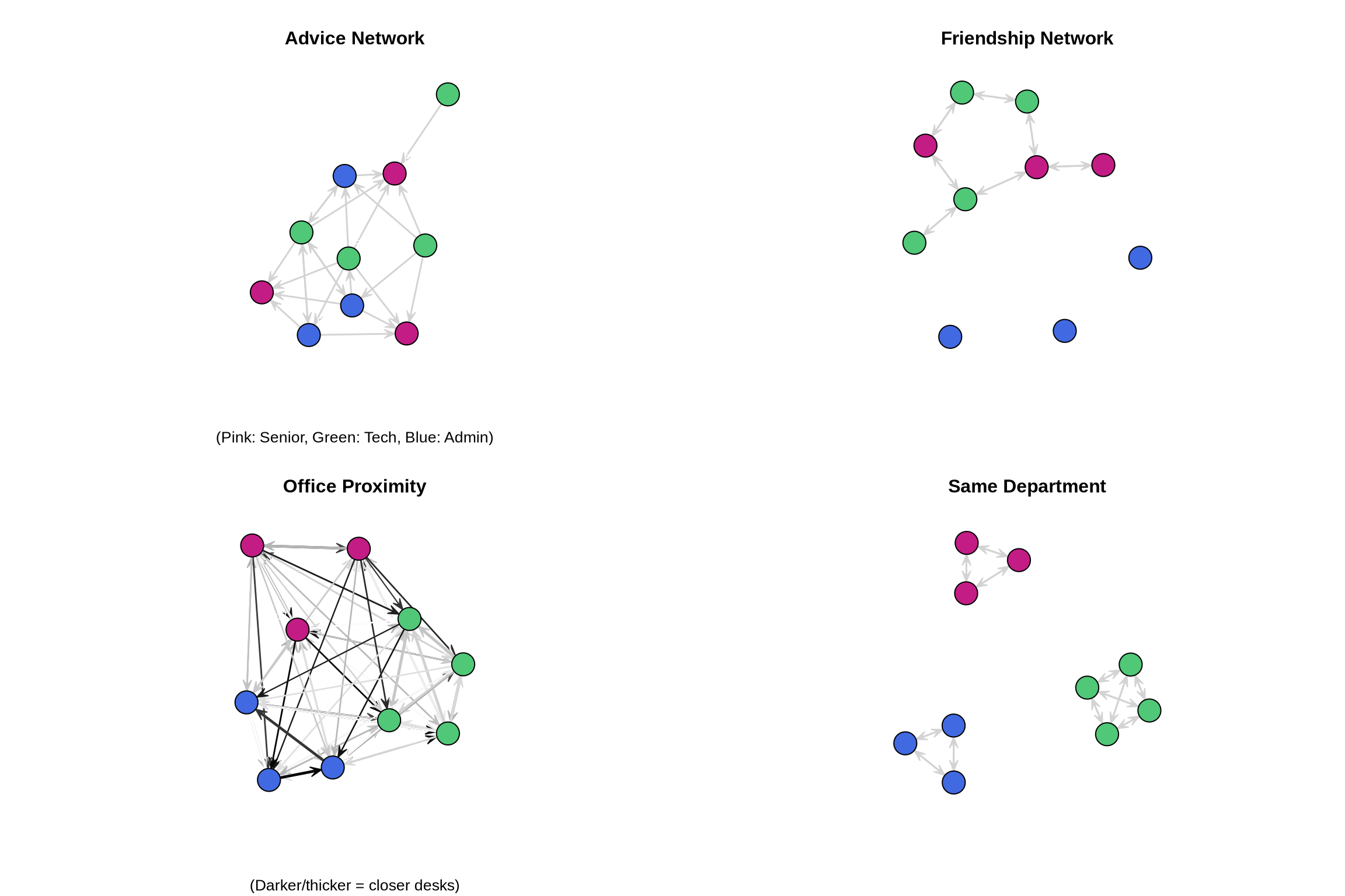

Part 3: QAP Correlation

Test pairwise correlations between networks using QAP:

# Test correlation between advice and friendship
qap_advice_friend <- qaptest(list(advice, friendship), 
                              gcor,
                              g1 = 1, g2 = 2,
                              reps = 1000)

cat("QAP Correlation: Advice ~ Friendship\n")

QAP Correlation: Advice ~ Friendship

cat("Observed correlation:", round(qap_advice_friend$testval, 3), "\n")

Observed correlation: -0.12 

cat("P-value:", round(qap_advice_friend$pgreq, 3), "\n\n")

P-value: 0.937 

# Visualize QAP test
hist(qap_advice_friend$dist, 
     breaks = 30,
     main = "QAP Test: Advice ~ Friendship",
     xlab = "Correlation",
     col = "lightgray")
abline(v = qap_advice_friend$testval, col = "red", lwd = 2)
text(qap_advice_friend$testval, max(table(cut(qap_advice_friend$dist, 30))), 
     "Observed", col = "red", pos = 4)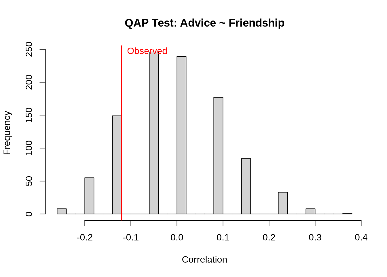

TipInterpretation

The QAP test permutes one matrix while holding the other fixed, maintaining the dependency structure. If p < 0.05, the correlation is significant.

# Test all pairwise correlations
networks <- list(advice, friendship, office_dist, same_dept)
net_names <- c("Advice", "Friendship", "Office", "SameDept")

# Create correlation matrix
qap_cors <- matrix(NA, 4, 4)
qap_pvals <- matrix(NA, 4, 4)

for(i in 1:4) {
  for(j in 1:4) {
    if(i != j) {
      qap_result <- qaptest(networks, gcor, g1 = i, g2 = j, reps = 500)
      qap_cors[i,j] <- qap_result$testval
      qap_pvals[i,j] <- qap_result$pgreq
    }
  }
}

# Display results
colnames(qap_cors) <- rownames(qap_cors) <- net_names
colnames(qap_pvals) <- rownames(qap_pvals) <- net_names

cat("\nQAP Correlation Matrix:\n")

QAP Correlation Matrix:

print(round(qap_cors, 3))

           Advice Friendship Office SameDept
Advice         NA     -0.120 -0.346   -0.364
Friendship -0.120         NA  0.132    0.157
Office     -0.346      0.132     NA    0.963
SameDept   -0.364      0.157  0.963       NA

cat("\nQAP P-values:\n")

QAP P-values:

print(round(qap_pvals, 3))

           Advice Friendship Office SameDept
Advice         NA      0.936  1.000    1.000
Friendship  0.940         NA  0.228    0.294
Office      0.998      0.226     NA    0.000
SameDept    1.000      0.276  0.002       NA

Part 4: QAP Regression

Now let’s predict advice-seeking from friendship, office proximity, and department:

# Prepare matrices for regression
y <- advice
X <- array(dim = c(3, n, n))
X[1,,] <- friendship
X[2,,] <- office_dist  
X[3,,] <- same_dept

# Run QAP regression with OLS
qap_ols <- netlm(y, X, 
                 mode = "digraph",
                 nullhyp = "qap",
                 reps = 1000)

# Display results
cat("QAP Regression Results: Advice Network\n")

QAP Regression Results: Advice Network

cat("=====================================\n")

=====================================

summary(qap_ols)

OLS Network Model

Residuals:
         0%         25%         50%         75%        100% 
-0.38036458 -0.37118013 -0.02597158  0.61973275  0.70609565 

Coefficients:
            Estimate    Pr(<=b) Pr(>=b) Pr(>=|b|)
(intercept)  0.36359484 0.998   0.002   0.002    
x1          -0.07784050 0.269   0.731   0.520    
x2           0.05628842 0.515   0.485   0.922    
x3          -0.39280897 0.166   0.834   0.329    

Residual standard error: 0.4204 on 86 degrees of freedom
Multiple R-squared: 0.1364  Adjusted R-squared: 0.1063 
F-statistic: 4.529 on 3 and 86 degrees of freedom, p-value: 0.005367 


Test Diagnostics:

    Null Hypothesis: qap 
    Replications: 1000 
    Coefficient Distribution Summary:

       (intercept)        x1        x2        x3
Min      -2.554932 -2.755432 -3.543105 -2.941607
1stQ     -0.011421 -0.682755 -0.642629 -0.720567
Median    0.647864 -0.056711  0.062208 -0.026336
Mean      0.651294 -0.022526  0.035152  0.006521
3rdQ      1.339457  0.629649  0.747231  0.724377
Max       4.194518  3.752002  3.602831  4.011717

NoteUnderstanding QAP Regression Output

• Coefficients: Effect of each predictor on advice-seeking
• Std. Error: Uncertainty in estimates
• P-values: Significance based on QAP permutations
• R-squared: Proportion of variance explained

Part 5: Visualizing Regression Results

# Extract coefficients and create bar plot
coef_names <- c("Intercept", "Friendship", "Office Proximity", "Same Dept")
coef_vals <- qap_ols$coefficients
coef_pvals <- qap_ols$pgreqabs

# Create coefficient plot
par(mfrow = c(2, 1))

# Coefficient values
barplot(coef_vals, 
        names.arg = coef_names,
        col = ifelse(coef_pvals < 0.05, "#c41c85", "gray"),
        main = "QAP Regression Coefficients",
        ylab = "Coefficient Value",
        las = 2)
abline(h = 0, lty = 2)
legend("topright", 
       legend = c("p < 0.05", "p ≥ 0.05"),
       fill = c("#c41c85", "gray"))

# P-values
barplot(-log10(coef_pvals), 
        names.arg = coef_names,
        col = ifelse(coef_pvals < 0.05, "#50C878", "lightgray"),
        main = "Statistical Significance (-log10 p-value)",
        ylab = "-log10(p-value)",
        las = 2)
abline(h = -log10(0.05), lty = 2, col = "red")
text(4, -log10(0.05), "p = 0.05", col = "red", pos = 3)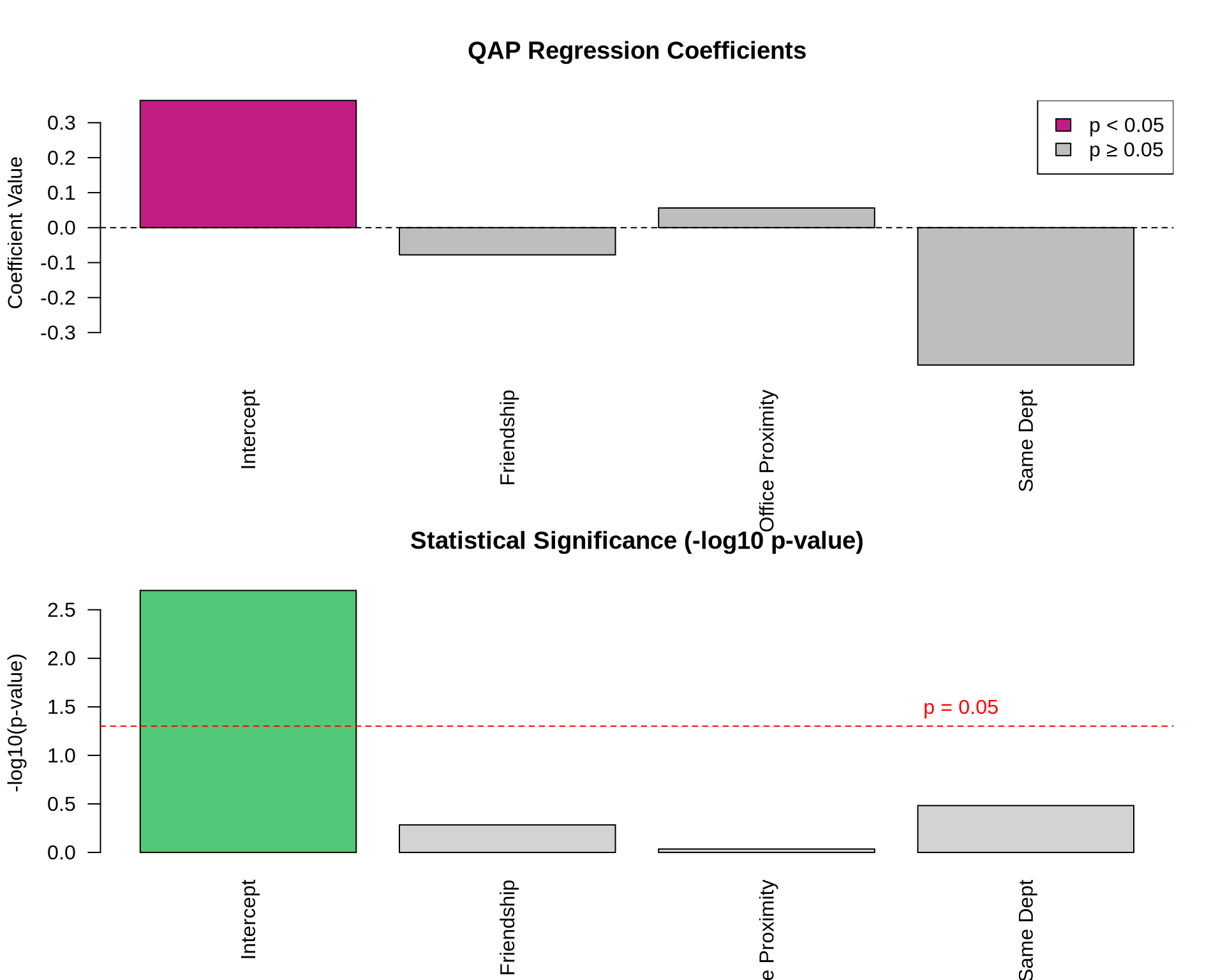

Part 6: Model Diagnostics

# Calculate fitted values and residuals
fitted_vals <- qap_ols$fitted.values
residuals <- qap_ols$residuals

# Residual plots
par(mfrow = c(1, 2))

# Histogram of residuals
hist(residuals, 
     breaks = 30,
     main = "Distribution of Residuals",
     xlab = "Residuals",
     col = "lightblue")

# Fitted vs residuals
plot(fitted_vals, residuals,
     main = "Fitted vs Residuals",
     xlab = "Fitted Values",
     ylab = "Residuals",
     pch = 19,
     col = rgb(0, 0, 0, 0.5))
abline(h = 0, col = "red", lty = 2)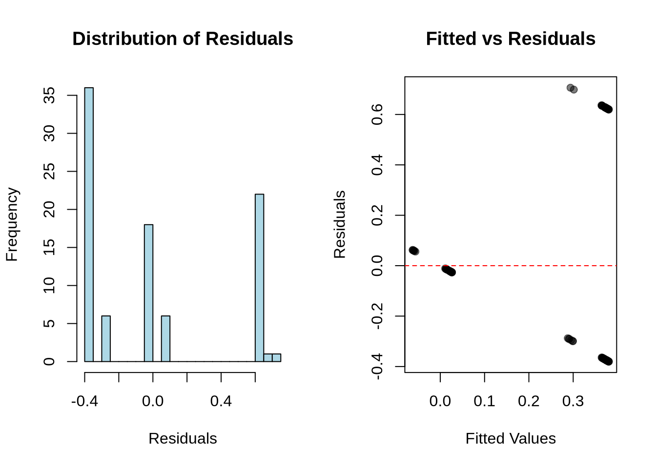

Your Turn

Try these exercises:

# Exercise 1: Create and test a hypothesis
# Do people seek advice more from those in their department who are also friends?
# Hint: Create an interaction term

# Your code here


# Exercise 2: Reverse the analysis
# Predict friendship from advice-seeking, proximity, and department

# Your code here


# Exercise 3: Add a new predictor
# Create a "seniority difference" matrix and add it to the model

# Your code here

Key Concepts

1. QAP preserves network structure during permutation tests
2. Network autocorrelation makes standard tests invalid
3. Multiple regression with QAP allows complex hypotheses
4. Effect sizes matter as much as significance

WarningCommon Pitfalls

• Don’t use standard correlation/regression on network data
• Check for multicollinearity between predictors
• Consider directed vs undirected relationships
• Remember that QAP is computationally intensive

NoteSolutions to Exercises

# Exercise 1 Solution: Interaction term
interaction <- friendship * same_dept
X_int <- array(dim = c(4, n, n))
X_int[1,,] <- friendship
X_int[2,,] <- office_dist
X_int[3,,] <- same_dept
X_int[4,,] <- interaction

qap_interact <- netlm(y, X_int, mode = "digraph", 
                      nullhyp = "qap", reps = 500)
summary(qap_interact)

# Exercise 2 Solution: Reverse prediction
y_friend <- friendship
X_friend <- array(dim = c(3, n, n))
X_friend[1,,] <- advice
X_friend[2,,] <- office_dist
X_friend[3,,] <- same_dept

qap_friend <- netlm(y_friend, X_friend, mode = "graph",
                    nullhyp = "qap", reps = 500)
summary(qap_friend)

# Exercise 3 Solution: Seniority difference
seniority <- c(10, 9, 8, 5, 4, 3, 3, 2, 1, 1)  # years
sen_diff <- matrix(0, n, n)
for(i in 1:n) {
  for(j in 1:n) {
    sen_diff[i,j] <- abs(seniority[i] - seniority[j])
  }
}

X_sen <- array(dim = c(4, n, n))
X_sen[1,,] <- friendship
X_sen[2,,] <- office_dist  
X_sen[3,,] <- same_dept
X_sen[4,,] <- sen_diff

qap_sen <- netlm(y, X_sen, mode = "digraph",
                 nullhyp = "qap", reps = 500)
summary(qap_sen)