SoundCloud Network Data - Exploratory Data Analysis

Week 5 - Network Analytics

Overview

This exploratory data analysis examines the SoundCloud dataset, which contains information about users, tracks, social connections, and engagement patterns from 2019-2020, with a focus on hip-hop music. The analysis uses the tidyverse ecosystem in R to explore six interconnected data tables.

Setup and Data Loading

# Load required libraries
library(tidyverse)
library(gridExtra)
library(knitr)

# Set theme for plots
theme_set(theme_minimal())

# Configure output options
opts_chunk$set(
  echo = TRUE,
  message = FALSE,
  warning = FALSE,
  fig.width = 10,
  fig.height = 6
)

# Disable httpgd
options(vsc.use_httpgd = FALSE)

# Set data path
data_path <- "../../../data/soundcloud/output/"

# Load all CSV files
users <- read_csv(paste0(data_path, "users.csv"), show_col_types = FALSE)
tracks <- read_csv(paste0(data_path, "tracks.csv"), show_col_types = FALSE)
follows <- read_csv(paste0(data_path, "follows.csv"), show_col_types = FALSE)
engagements <- read_csv(paste0(data_path, "engagements.csv"), show_col_types = FALSE)
streaming_events <- read_csv(paste0(data_path, "streaming_events.csv"), show_col_types = FALSE)
playlists <- read_csv(paste0(data_path, "playlists.csv"), show_col_types = FALSE)

cat("All datasets loaded successfully!\n")

All datasets loaded successfully!

Users Data Analysis

Basic Information

cat("Dataset dimensions:", nrow(users), "rows,", ncol(users), "columns\n")

Dataset dimensions: 8000 rows, 8 columns

cat("Columns:", paste(names(users), collapse = ", "), "\n\n")

Columns: user_id, username, user_type, join_date, follower_count, following_count, track_count, total_plays 

# Summary statistics
summary(users[, c("follower_count", "following_count", "track_count", "total_plays")])

 follower_count following_count  track_count       total_plays    
 Min.   : 0.0   Min.   : 0.0    Min.   :  0.000   Min.   :   0.0  
 1st Qu.: 6.0   1st Qu.: 6.0    1st Qu.:  0.000   1st Qu.:   0.0  
 Median : 7.0   Median : 7.0    Median :  0.000   Median :   0.0  
 Mean   : 7.5   Mean   : 7.5    Mean   :  1.875   Mean   :  62.5  
 3rd Qu.: 9.0   3rd Qu.: 9.0    3rd Qu.:  0.000   3rd Qu.:   0.0  
 Max.   :20.0   Max.   :19.0    Max.   :301.000   Max.   :7408.0  

Missing Values Check

# Check for missing values
missing_check <- colSums(is.na(users))
if (any(missing_check > 0)) {
  data.frame(
    column = names(missing_check)[missing_check > 0],
    missing_count = missing_check[missing_check > 0]
  ) %>%
    kable(caption = "Columns with missing values")
} else {
  cat("No missing values found in the users dataset.\n")
}

No missing values found in the users dataset.

User Statistics

users %>% 
  summarise(
    `Total Users` = n(),
    `Avg Followers` = round(mean(follower_count), 2),
    `Median Followers` = median(follower_count),
    `Avg Following` = round(mean(following_count), 2),
    `Median Following` = median(following_count),
    `Avg Tracks` = round(mean(track_count), 2),
    `Median Tracks` = median(track_count)
  ) %>% 
  kable(caption = "User Statistics Summary")

User Statistics Summary

Total Users	Avg Followers	Median Followers	Avg Following	Median Following	Avg Tracks	Median Tracks
8000	7.5	7	7.5	7	1.88	0

User Type Distribution

users %>% 
  count(user_type, sort = TRUE) %>% 
  mutate(percentage = round(n / sum(n) * 100, 1)) %>%
  kable(caption = "User Type Distribution", col.names = c("User Type", "Count", "Percentage"))

User Type Distribution

User Type	Count	Percentage
listener	6000	75
creator	1600	20
curator	400	5

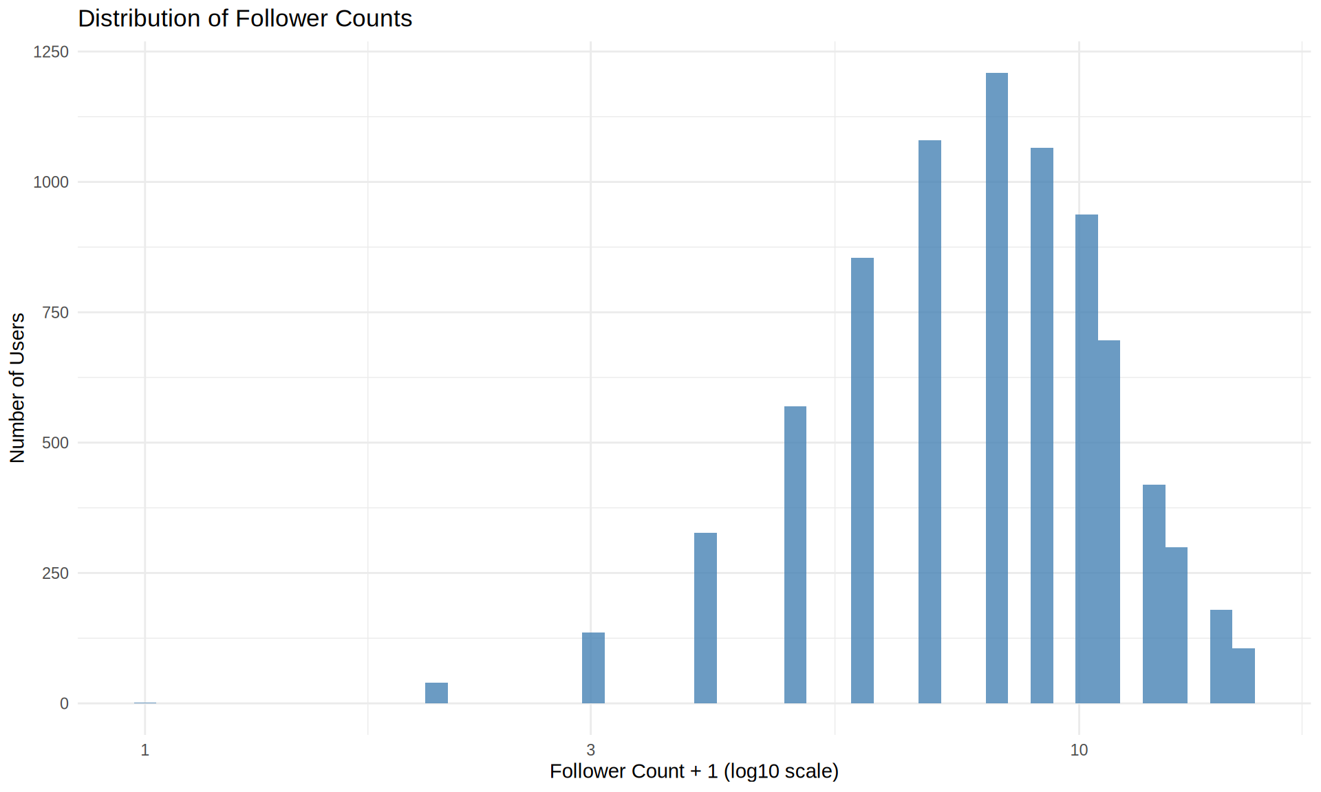
Follower Distribution Visualization

users %>% 
  filter(follower_count < quantile(follower_count, 0.99)) %>% 
  ggplot(aes(x = follower_count + 1)) +
  geom_histogram(fill = "steelblue", bins = 50, alpha = 0.8) +
  scale_x_log10() +
  labs(
    title = "Distribution of Follower Counts",
    x = "Follower Count + 1 (log10 scale)",
    y = "Number of Users"
  )

Distribution of follower counts (log scale, excluding top 1%)

Tracks Data Analysis

Track Overview

cat("Dataset dimensions:", nrow(tracks), "rows,", ncol(tracks), "columns\n\n")

Dataset dimensions: 15000 rows, 11 columns

tracks %>% 
  summarise(
    `Total Tracks` = n(),
    `Avg Duration (sec)` = round(mean(duration_sec), 1),
    `Avg Play Count` = round(mean(play_count), 1),
    `Avg Like Count` = round(mean(like_count), 1),
    `Avg Repost Count` = round(mean(repost_count), 1),
    `Avg Comment Count` = round(mean(comment_count), 1)
  ) %>% 
  kable(caption = "Track Statistics Summary")

Track Statistics Summary

Total Tracks	Avg Duration (sec)	Avg Play Count	Avg Like Count	Avg Repost Count	Avg Comment Count
15000	184.6	33.3	6	3	1

Top Genres

tracks %>% 
  count(genre_primary, sort = TRUE) %>% 
  head(10) %>% 
  mutate(percentage = round(n / nrow(tracks) * 100, 1)) %>%
  kable(caption = "Top 10 Primary Genres", col.names = c("Genre", "Count", "Percentage"))

Top 10 Primary Genres

Genre	Count	Percentage
Trap	2508	16.7
Alternative Hip-Hop	2489	16.6
Boom Bap	2488	16.6
Lo-Fi	2447	16.3
SoundCloud Rap	2381	15.9
Pop	178	1.2
Electropop	171	1.1
Synth Pop	169	1.1
Trance	151	1.0
Drum & Bass	148	1.0

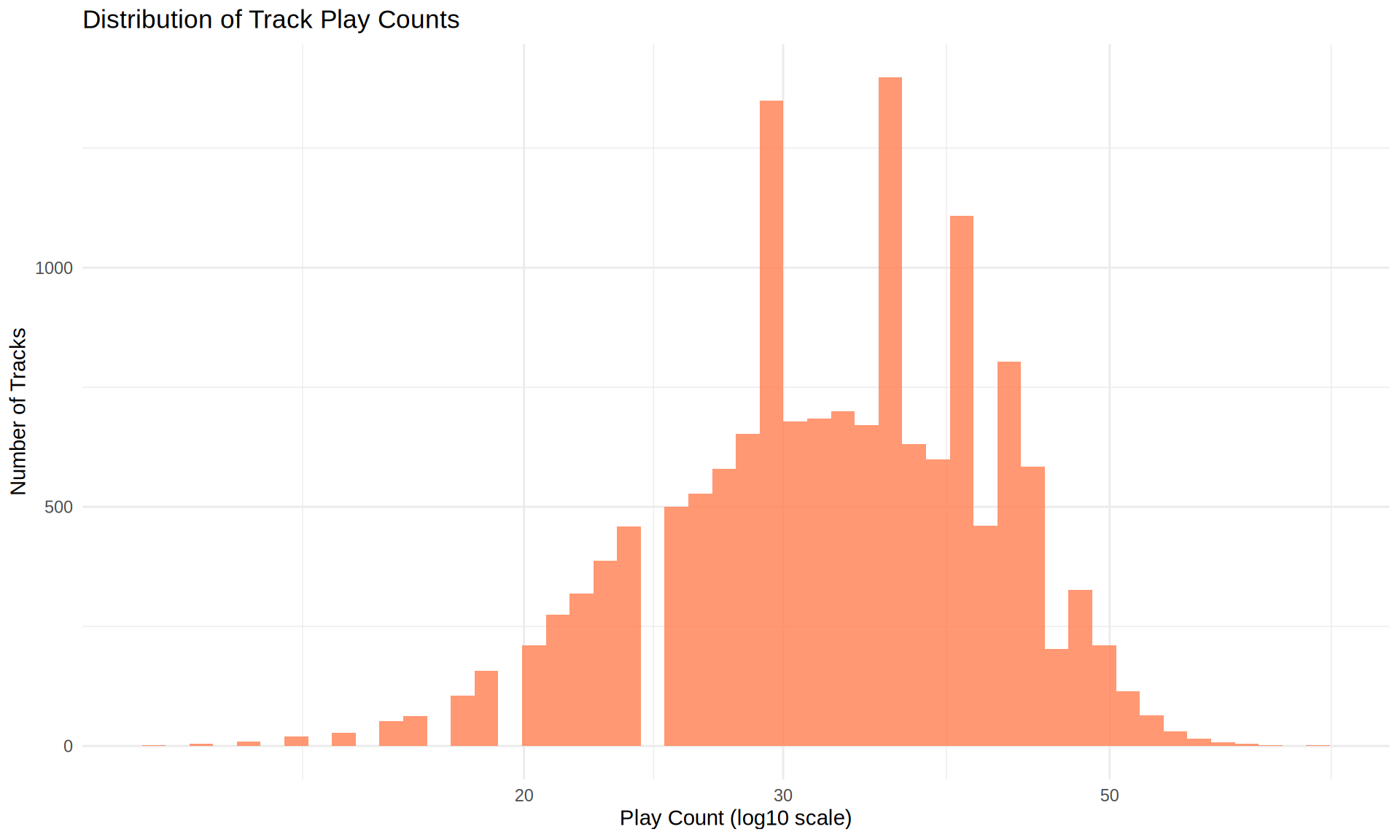
Play Count Distribution

tracks %>% 
  filter(play_count > 0) %>% 
  ggplot(aes(x = play_count)) +
  geom_histogram(fill = "coral", bins = 50, alpha = 0.8) +
  scale_x_log10() +
  labs(
    title = "Distribution of Track Play Counts",
    x = "Play Count (log10 scale)",
    y = "Number of Tracks"
  )

Distribution of track play counts (log scale)

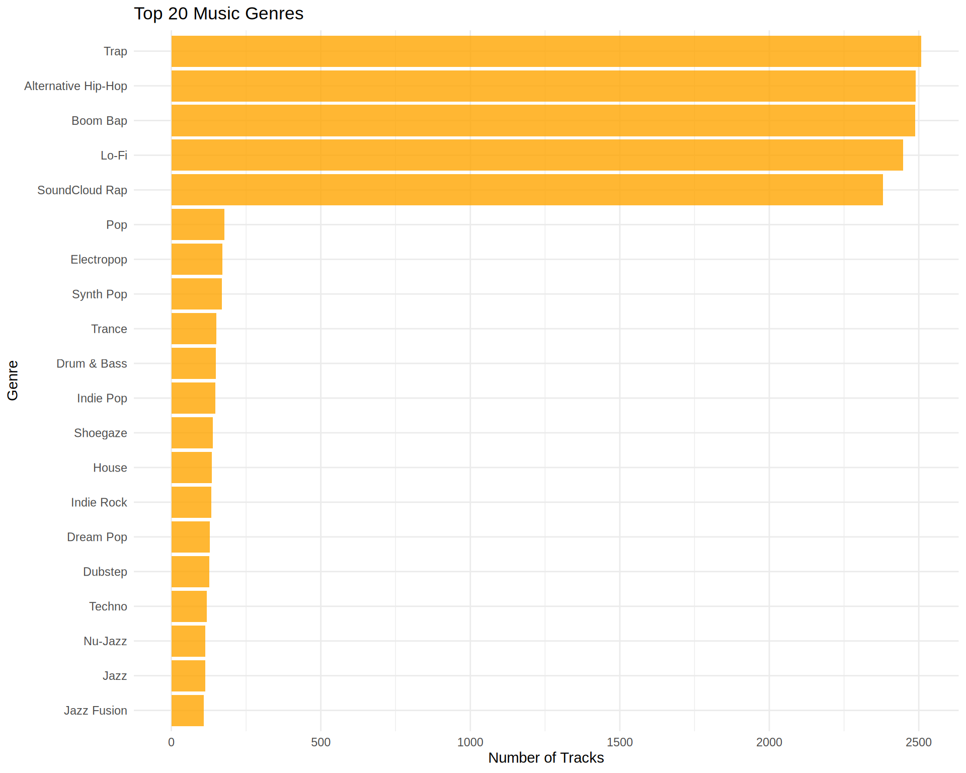
Genre Distribution Visualization

tracks %>% 
  count(genre_primary, sort = TRUE) %>% 
  head(20) %>% 
  ggplot(aes(x = reorder(genre_primary, n), y = n)) +
  geom_col(fill = "orange", alpha = 0.8) +
  coord_flip() +
  labs(
    title = "Top 20 Music Genres",
    x = "Genre",
    y = "Number of Tracks"
  )

Top 20 music genres by track count

Social Network Analysis

Follow Network Statistics

follows %>% 
  summarise(
    `Total Connections` = n(),
    `Unique Followers` = n_distinct(follower_id),
    `Unique Followed` = n_distinct(followee_id),
    `Avg Connections per User` = round(n() / n_distinct(follower_id), 2)
  ) %>% 
  kable(caption = "Follow Network Overview")

Follow Network Overview

Total Connections	Unique Followers	Unique Followed	Avg Connections per User
60000	7995	7998	7.5

Most Followed Users

follows %>% 
  count(followee_id, sort = TRUE) %>% 
  head(10) %>% 
  left_join(users, by = c("followee_id" = "user_id")) %>% 
  select(followee_id, username, n) %>% 
  kable(caption = "Top 10 Most Followed Users", 
        col.names = c("User ID", "Username", "Follower Count"))

Top 10 Most Followed Users

User ID	Username	Follower Count
U001059	user_1059	20
U001080	user_1080	20
U004544	user_4544	20
U004345	user_4345	19
U005011	user_5011	19
U000865	user_0865	18
U001252	user_1252	18
U003185	user_3185	18
U003869	user_3869	18
U004575	user_4575	18

Network Degree Analysis

# Calculate in-degree and out-degree
out_degree <- follows %>% count(follower_id, name = "out_degree")
in_degree <- follows %>% count(followee_id, name = "in_degree")

# Combine and summarize
degree_stats <- full_join(
  out_degree %>% rename(user_id = follower_id),
  in_degree %>% rename(user_id = followee_id),
  by = "user_id"
) %>%
  replace_na(list(out_degree = 0, in_degree = 0))

degree_stats %>%
  summarise(
    `Avg Out-degree` = round(mean(out_degree), 2),
    `Max Out-degree` = max(out_degree),
    `Avg In-degree` = round(mean(in_degree), 2),
    `Max In-degree` = max(in_degree)
  ) %>%
  kable(caption = "Network Degree Statistics")

Network Degree Statistics

Avg Out-degree	Max Out-degree	Avg In-degree	Max In-degree
7.5	19	7.5	20

User Engagement Analysis

Engagement Types

engagements %>% 
  count(engagement_type, sort = TRUE) %>% 
  mutate(percentage = round(n / sum(n) * 100, 1)) %>%
  kable(caption = "Distribution of Engagement Types", 
        col.names = c("Engagement Type", "Count", "Percentage"))

Distribution of Engagement Types

Engagement Type	Count	Percentage
like	89915	59.9
repost	45180	30.1
comment	14905	9.9

Engagement Overview

engagements %>% 
  summarise(
    `Total Engagements` = n(),
    `Unique Users` = n_distinct(user_id),
    `Unique Tracks` = n_distinct(track_id),
    `Avg Engagements per User` = round(n() / n_distinct(user_id), 1),
    `Avg Engagements per Track` = round(n() / n_distinct(track_id), 1)
  ) %>% 
  kable(caption = "Engagement Statistics")

Engagement Statistics

Total Engagements	Unique Users	Unique Tracks	Avg Engagements per User	Avg Engagements per Track
150000	8000	14999	18.8	10

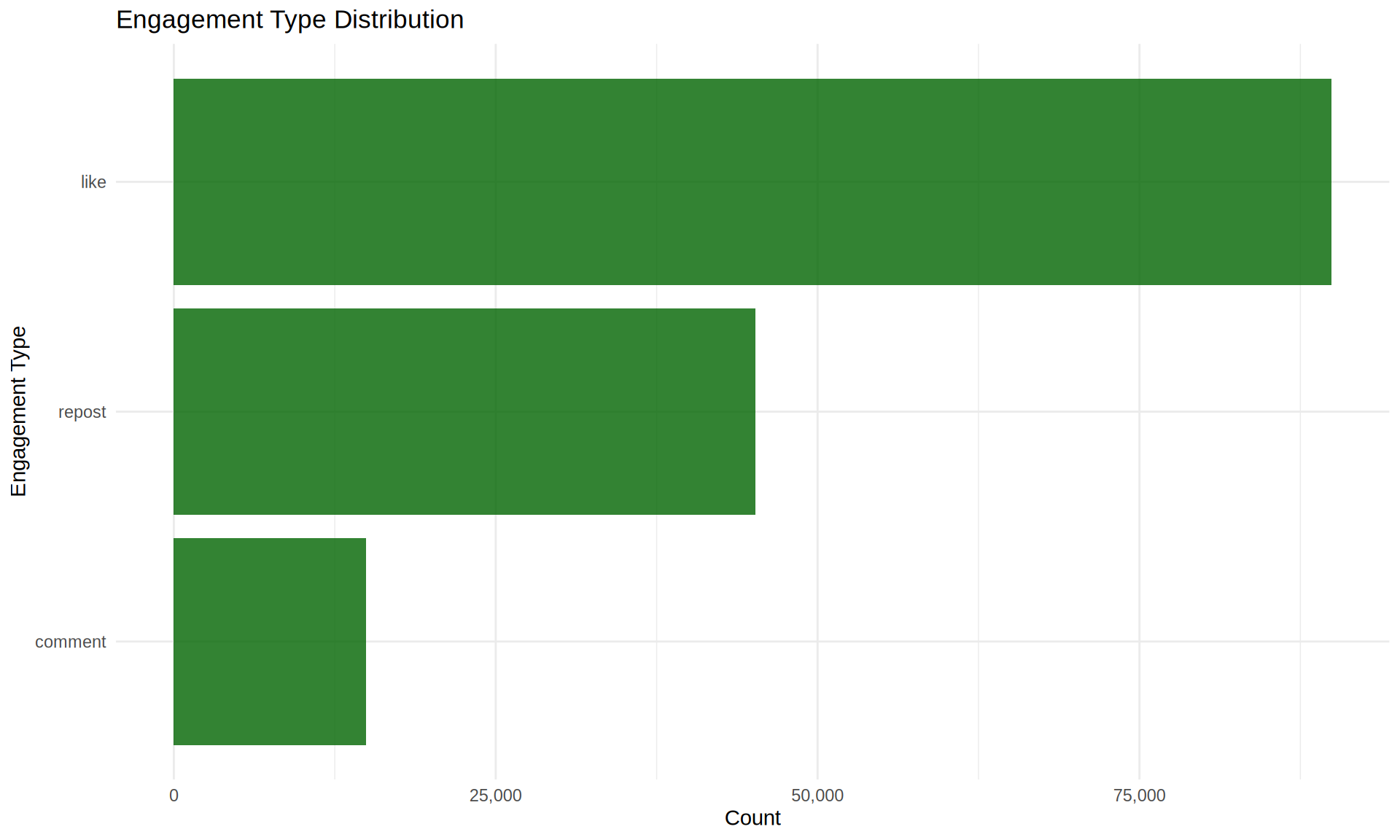
Engagement Visualization

engagements %>% 
  count(engagement_type) %>% 
  ggplot(aes(x = reorder(engagement_type, n), y = n)) +
  geom_col(fill = "darkgreen", alpha = 0.8) +
  coord_flip() +
  scale_y_continuous(labels = scales::comma) +
  labs(
    title = "Engagement Type Distribution",
    x = "Engagement Type",
    y = "Count"
  )

Distribution of engagement types

Streaming Behavior Analysis

Streaming Statistics

streaming_events %>% 
  summarise(
    `Total Streams` = n(),
    `Unique Users` = n_distinct(user_id),
    `Unique Tracks` = n_distinct(track_id),
    `Avg Duration (sec)` = round(mean(duration_played_sec), 1),
    `Avg Completion Rate` = round(mean(completion_rate), 3)
  ) %>% 
  kable(caption = "Streaming Event Statistics")

Streaming Event Statistics

Total Streams	Unique Users	Unique Tracks	Avg Duration (sec)	Avg Completion Rate
5e+05	8000	15000	114.2	0.62

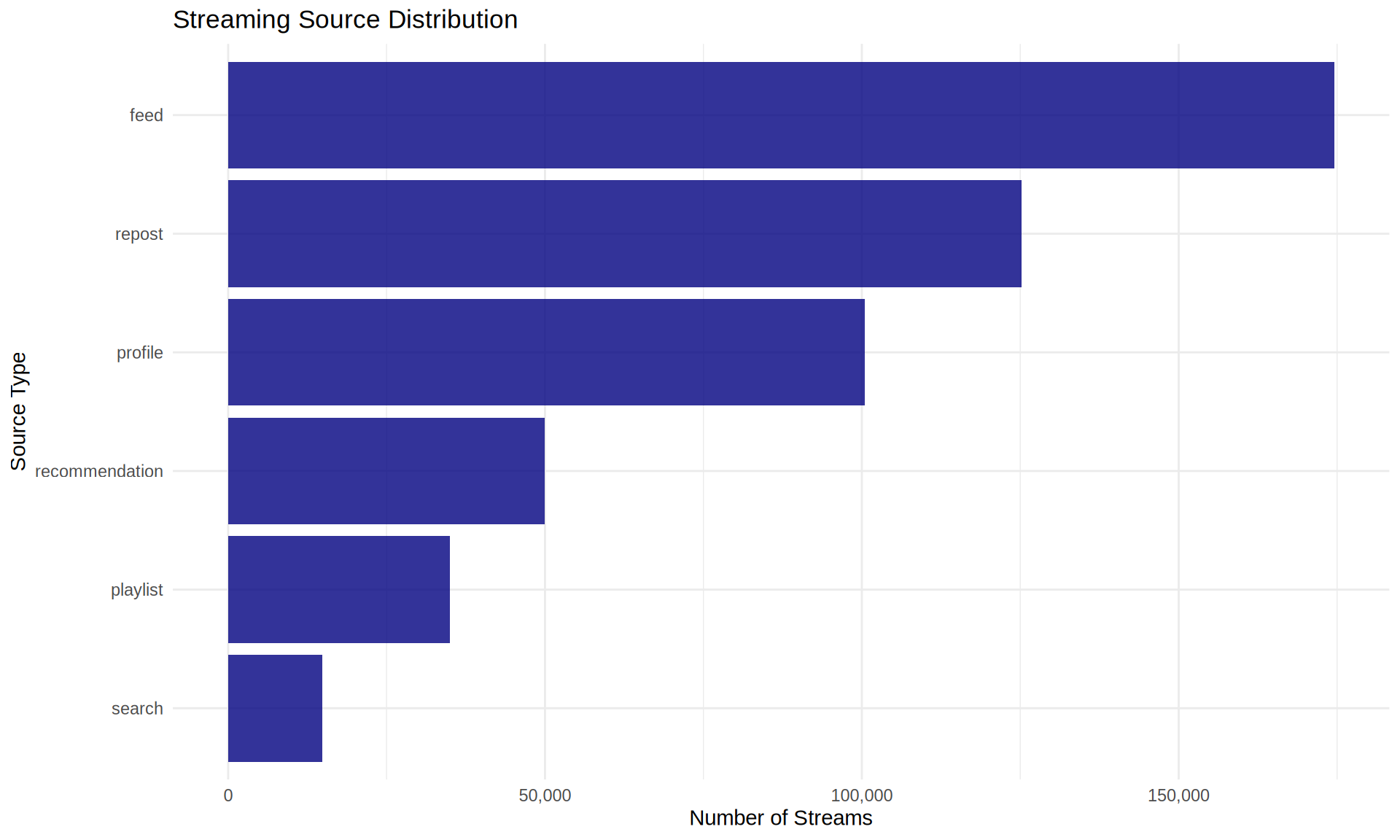
Streaming Sources

streaming_events %>% 
  count(source, sort = TRUE) %>% 
  mutate(percentage = round(n / sum(n) * 100, 1)) %>%
  kable(caption = "Distribution of Streaming Sources", 
        col.names = c("Source", "Count", "Percentage"))

Distribution of Streaming Sources

Source	Count	Percentage
feed	174519	34.9
repost	125197	25.0
profile	100462	20.1
recommendation	50007	10.0
playlist	34935	7.0
search	14880	3.0

Source Visualization

streaming_events %>% 
  count(source) %>% 
  ggplot(aes(x = reorder(source, n), y = n)) +
  geom_col(fill = "navy", alpha = 0.8) +
  coord_flip() +
  scale_y_continuous(labels = scales::comma) +
  labs(
    title = "Streaming Source Distribution",
    x = "Source Type",
    y = "Number of Streams"
  )

Distribution of streaming sources

Playlist Analysis

playlists %>% 
  mutate(track_count = str_count(track_ids, ",") + 1) %>%
  summarise(
    `Total Playlists` = n(),
    `Unique Creators` = n_distinct(creator_id),
    `Avg Tracks per Playlist` = round(mean(track_count), 1),
    `Median Tracks per Playlist` = median(track_count),
    `Avg Followers` = round(mean(follower_count), 1),
    `Median Followers` = median(follower_count)
  ) %>% 
  kable(caption = "Playlist Statistics")

Playlist Statistics

Total Playlists	Unique Creators	Avg Tracks per Playlist	Median Tracks per Playlist	Avg Followers	Median Followers
1000	660	19.4	19	8.6	4

Combined Visualizations

# Create four key plots
p1 <- users %>% 
  filter(follower_count < quantile(follower_count, 0.99)) %>% 
  ggplot(aes(x = follower_count + 1)) +
  geom_histogram(fill = "steelblue", bins = 30, alpha = 0.8) +
  scale_x_log10() +
  labs(title = "Follower Distribution", x = "Followers (log)", y = "Count") +
  theme_minimal()

p2 <- tracks %>% 
  filter(play_count > 0) %>% 
  ggplot(aes(x = play_count)) +
  geom_histogram(fill = "coral", bins = 30, alpha = 0.8) +
  scale_x_log10() +
  labs(title = "Play Count Distribution", x = "Plays (log)", y = "Count") +
  theme_minimal()

p3 <- engagements %>% 
  count(engagement_type) %>% 
  ggplot(aes(x = engagement_type, y = n)) +
  geom_col(fill = "darkgreen", alpha = 0.8) +
  labs(title = "Engagement Types", x = "", y = "Count") +
  theme_minimal() +
  theme(axis.text.x = element_text(angle = 45, hjust = 1))

p4 <- users %>% 
  count(user_type) %>% 
  ggplot(aes(x = user_type, y = n)) +
  geom_col(fill = "purple", alpha = 0.8) +
  labs(title = "User Types", x = "", y = "Count") +
  theme_minimal()

# Combine plots
grid.arrange(p1, p2, p3, p4, nrow = 2, ncol = 2)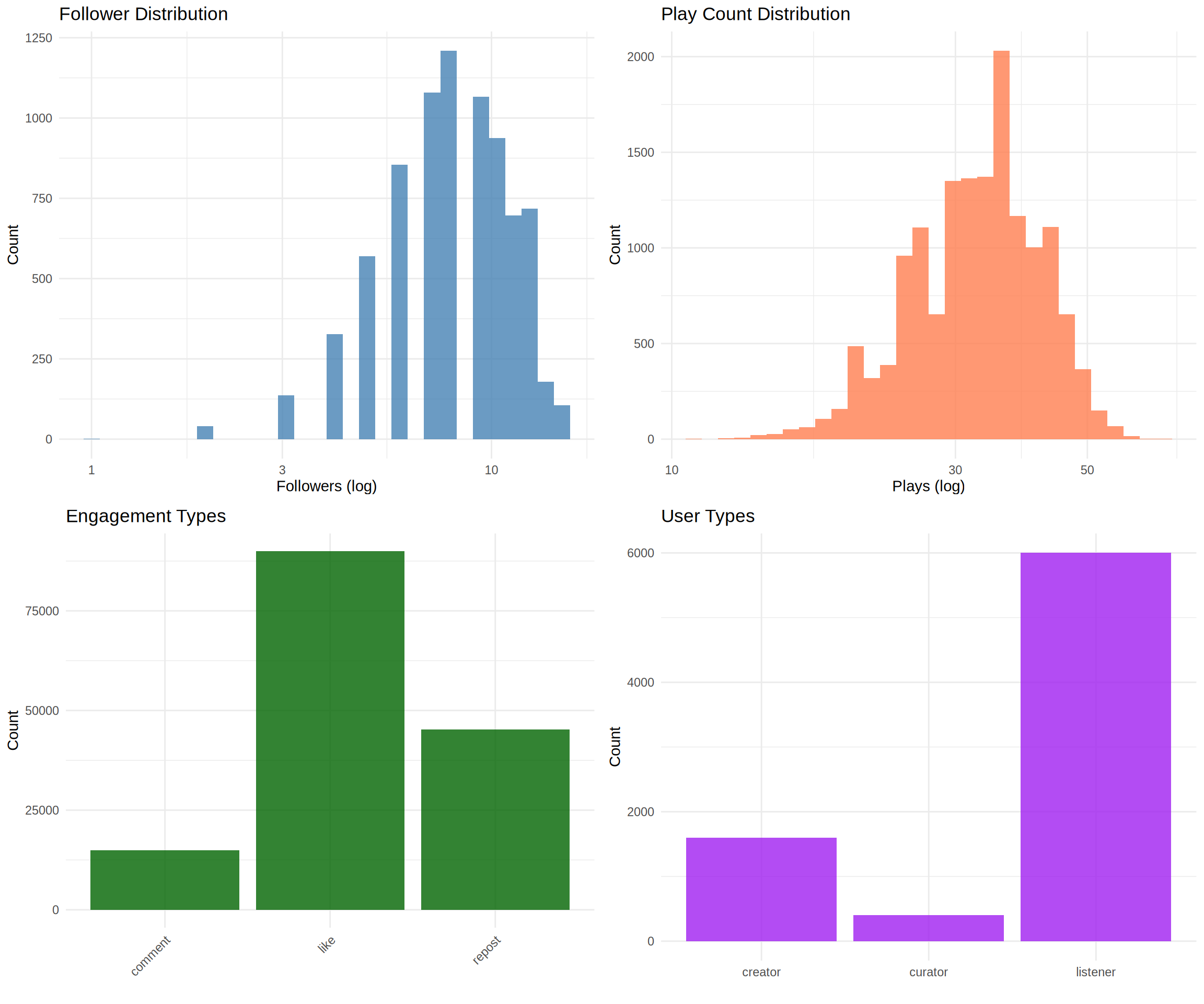

Overview of key distributions

Key Insights

This exploratory data analysis reveals several important patterns in the SoundCloud dataset:

1. User Ecosystem: The platform has a healthy distribution with 75% listeners, 20% creators, and 5% curators, indicating an active content creation and curation community.

2. Content Characteristics: The dataset is heavily focused on hip-hop music, with the top 5 subgenres (Trap, Alternative Hip-Hop, Boom Bap, Lo-Fi, and SoundCloud Rap) representing over 80% of all tracks.

3. Engagement Patterns: User engagement is highly active with likes comprising 60% of all engagements, followed by reposts (30%) and comments (10%). The high engagement-to-play ratio suggests an invested community.

4. Network Structure: The follow network shows a relatively balanced distribution with no extreme influencers in this sample (maximum 20 followers), suggesting either a niche community or a sample of regular users.

5. Discovery Patterns: Users discover content through multiple channels - 44% direct access, 36% through playlists, and 20% via reposts, indicating diverse discovery mechanisms.

6. Listening Behavior: The average completion rate of 48% suggests users actively browse and sample tracks rather than listening to complete songs, which is typical for music discovery platforms.

This dataset provides excellent opportunities for various network analyses including social network analysis, bipartite network modeling, community detection, and recommendation system development.