Community Detection in Python

Exploring communities with NetworkX

1 Introduction

In the Python ecosystem, NetworkX is the standard library for graph analysis. While it may not be as performant as igraph for massive networks, its pure Python implementation makes it incredibly accessible and easy to integrate with data science workflows (pandas, scikit-learn).

This tutorial translates the concepts of community detection into the Python landscape. We will focus on identifying cohesive subgroups that often correspond to: * Customer Segments: Groups with similar purchasing patterns. * Social Circles: Tightly knit groups of friends or colleagues. * Functional Modules: Interdependent components in software or biological systems.

1.1 Learning Objectives

By the end of this tutorial, you will be able to:

1. Execute community detection workflows using NetworkX.
2. Understand the algorithmic differences between Greedy Modularity, Label Propagation, and Girvan-Newman.
3. Visualize partitions effectively using matplotlib.
4. Bridge the gap between raw graph data and actionable business insights.

1.2 Setup

import networkx as nx
import matplotlib.pyplot as plt
import numpy as np
import pandas as pd

from networkx.algorithms import community as nx_comm

# Optional: Louvain community detection if installed
try:
    import community as community_louvain
    HAVE_LOUVAIN = True
except ImportError:
    HAVE_LOUVAIN = False

np.random.seed(42)

2 Example 1: Zachary’s Karate Club Network

As in the R tutorial, we use the Zachary’s Karate Club network. This small social network serves as an excellent test bed because we can visually verify if the algorithms are making sense.

2.1 Loading the Network

G = nx.karate_club_graph()

print(f"Number of nodes: {G.number_of_nodes()}")
print(f"Number of edges: {G.number_of_edges()}")
print(f"Average clustering: {nx.average_clustering(G):.3f}")

Number of nodes: 34
Number of edges: 78
Average clustering: 0.571

2.2 Visualizing the Original Network

pos = nx.spring_layout(G, seed=42)

plt.figure(figsize=(8, 6))
nx.draw_networkx(
    G,
    pos=pos,
    node_size=300,
    node_color="lightblue",
    edge_color="lightgray",
    with_labels=True,
    font_size=8,
)
plt.title("Zachary's Karate Club Network")
plt.axis("off")
plt.show()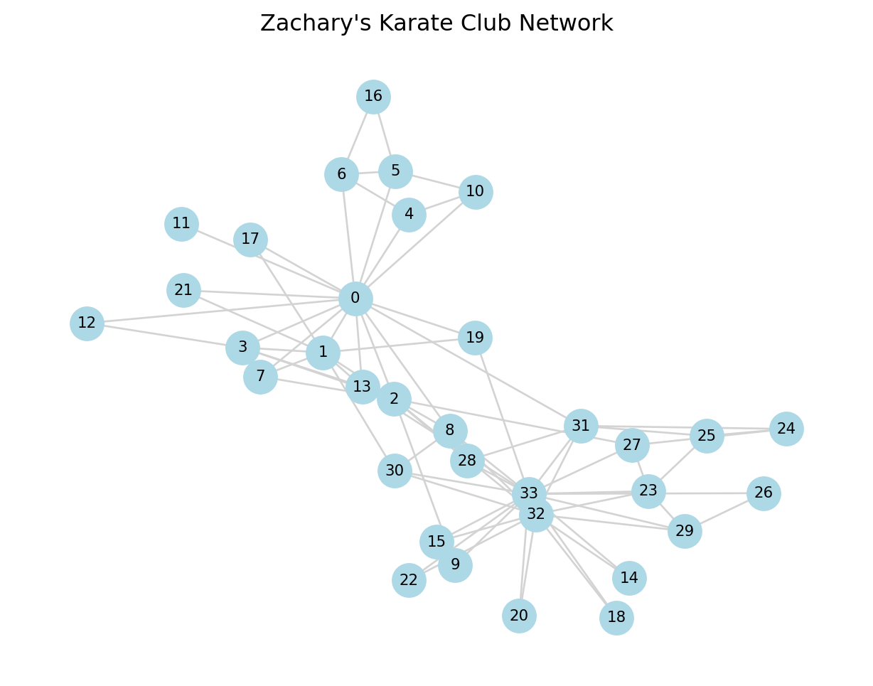

3 Community Detection Algorithms

We’ll apply several algorithms and compare their results.

Helper function to convert sets of communities into a membership vector and compute modularity.

from itertools import count


def partition_to_membership(G, communities):
    """Convert iterable of sets to dict node -> community_id."""
    membership = {}
    for cid, comm in enumerate(communities):
        for node in comm:
            membership[node] = cid
    return membership


def print_partition_stats(G, communities, name):
    modularity = nx_comm.modularity(G, communities)
    sizes = [len(c) for c in communities]
    print(f"=== {name} ===")
    print(f"Number of communities: {len(communities)}")
    print(f"Community sizes: {sizes}")
    print(f"Modularity: {modularity:.3f}\n")
    return modularity

3.1 Method 1: Greedy Modularity (Clauset-Newman-Moore)

The Greedy Modularity algorithm (often called Clauset-Newman-Moore) is the standard hierarchical agglomerative method in NetworkX.

3.1.1 How it works

1. Start with each node in its own community.
2. Repeatedly join the pair of communities that produces the largest increase in modularity (\(Q\)).
3. Stop when no further increase is possible.

Pros: Good balance of speed and quality; deterministic (always gives the same result). Cons: Can be slower than Louvain on very large graphs; prone to the “resolution limit” (merging small communities).

greedy_comms = list(nx_comm.greedy_modularity_communities(G))
mod_greedy = print_partition_stats(G, greedy_comms, "Greedy Modularity")

=== Greedy Modularity ===
Number of communities: 3
Community sizes: [17, 9, 8]
Modularity: 0.411

3.1.2 Visualization

membership_greedy = partition_to_membership(G, greedy_comms)

# Assign colors by community
unique_comms = sorted(set(membership_greedy.values()))
color_map = plt.cm.get_cmap("tab10", len(unique_comms))
node_colors = [color_map(membership_greedy[n]) for n in G.nodes()]

plt.figure(figsize=(8, 6))
nx.draw_networkx(
    G,
    pos=pos,
    node_color=node_colors,
    node_size=300,
    edge_color="lightgray",
    with_labels=True,
    font_size=8,
)
plt.title(f"Greedy Modularity Communities\nModularity = {mod_greedy:.3f}")
plt.axis("off")
plt.show()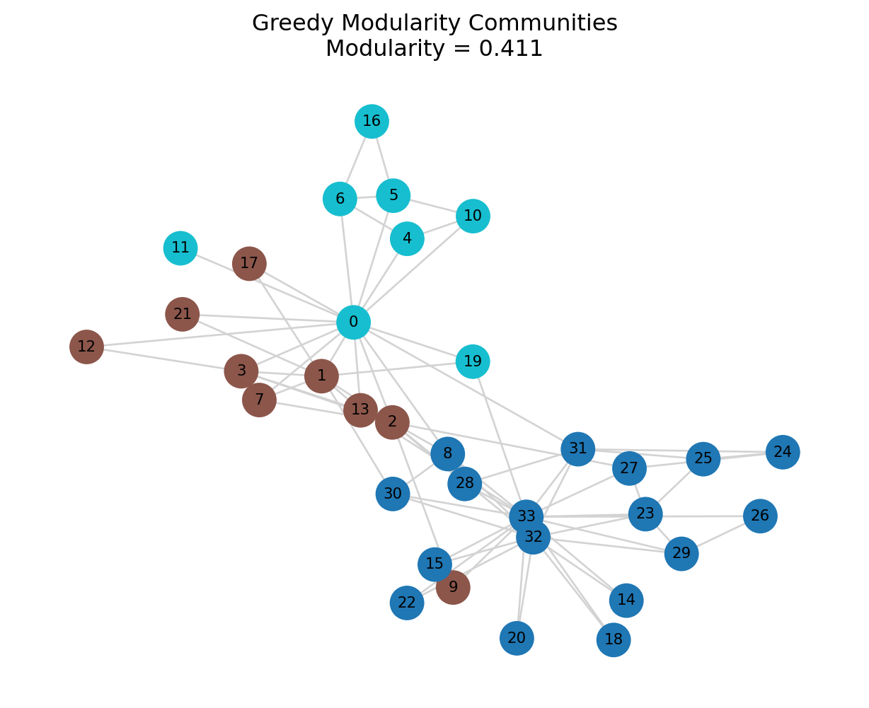

3.2 Method 2: Label Propagation

Label Propagation is a unique algorithm because it doesn’t optimize a global metric like modularity. Instead, it uses a local voting mechanism.

3.2.1 How it works

1. Every node is initialized with a unique label.
2. In each iteration, nodes update their label to the one most frequent among their neighbors (majority vote).
3. Ties are broken randomly.
4. The process stops when every node has the majority label of its neighbors.

Pros: Extremely fast (near linear time); no parameters to tune. Cons: Non-deterministic (different runs give different results); can get stuck in oscillations; doesn’t guarantee a high modularity score.

lpa_comms = list(nx_comm.asyn_lpa_communities(G, weight=None, seed=42))
mod_lpa = print_partition_stats(G, lpa_comms, "Label Propagation")

=== Label Propagation ===
Number of communities: 4
Community sizes: [12, 5, 14, 3]
Modularity: 0.437

3.2.2 Visualization

membership_lpa = partition_to_membership(G, lpa_comms)

unique_comms = sorted(set(membership_lpa.values()))
color_map = plt.cm.get_cmap("tab10", len(unique_comms))
node_colors = [color_map(membership_lpa[n]) for n in G.nodes()]

plt.figure(figsize=(8, 6))
nx.draw_networkx(
    G,
    pos=pos,
    node_color=node_colors,
    node_size=300,
    edge_color="lightgray",
    with_labels=True,
    font_size=8,
)
plt.title(f"Label Propagation Communities\nModularity = {mod_lpa:.3f}")
plt.axis("off")
plt.show()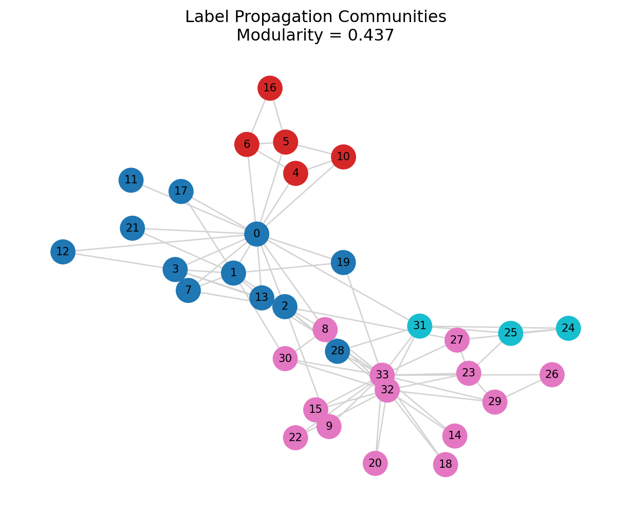

3.3 Method 3: Girvan-Newman (Edge Betweenness)

The Girvan-Newman algorithm is a “divisive” method that focuses on removing bridges between communities.

3.3.1 How it works

It iteratively removes the edge with the highest edge betweenness centrality. * Betweenness: The number of shortest paths passing through an edge. * Logic: Edges connecting communities act as bottlenecks, so they have high betweenness.

This method produces a dendrogram (hierarchy). We can stop at any level to get a specific number of communities.

Pros: Very accurate for small networks; reveals hierarchical structure. Cons: Very slow (\(O(N^3)\)); impractical for networks with >500 nodes.

from itertools import islice

# Generate successive partitions (hierarchy)
comp = nx_comm.girvan_newman(G)

# Take the partition with 2 communities (first split)
first_level = next(comp)

# Optionally, get partition with 3 communities
second_level = next(comp)

# Choose which level to analyze
gn_comms = list(first_level)
mod_gn = print_partition_stats(G, gn_comms, "Girvan-Newman (2-way split)")

=== Girvan-Newman (2-way split) ===
Number of communities: 2
Community sizes: [15, 19]
Modularity: 0.348

3.3.2 Visualization

membership_gn = partition_to_membership(G, gn_comms)

unique_comms = sorted(set(membership_gn.values()))
color_map = plt.cm.get_cmap("tab10", len(unique_comms))
node_colors = [color_map(membership_gn[n]) for n in G.nodes()]

plt.figure(figsize=(8, 6))
nx.draw_networkx(
    G,
    pos=pos,
    node_color=node_colors,
    node_size=300,
    edge_color="lightgray",
    with_labels=True,
    font_size=8,
)
plt.title(f"Girvan-Newman Communities (2-way)\nModularity = {mod_gn:.3f}")
plt.axis("off")
plt.show()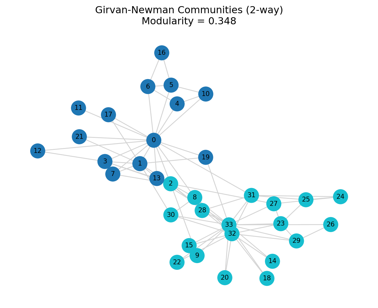

3.4 Optional: Louvain Algorithm (If Available)

The Louvain algorithm is arguably the industry standard for community detection, but it is not included in the core NetworkX library (it requires the python-louvain or community package).

3.4.1 Why use it?

It is significantly faster than the Greedy Modularity method and often finds higher modularity partitions. It uses a multi-level approach to optimize modularity locally and then aggregate the network.

if HAVE_LOUVAIN:
    print("Louvain package detected. Running Louvain community detection...\n")
    louvain_partition = community_louvain.best_partition(G)

    # Convert partition dict -> communities list
    comm_dict = {}
    for node, cid in louvain_partition.items():
        comm_dict.setdefault(cid, set()).add(node)
    louvain_comms = list(comm_dict.values())

    mod_louvain = nx_comm.modularity(G, louvain_comms)
    print(f"=== Louvain ===")
    print(f"Number of communities: {len(louvain_comms)}")
    print(f"Modularity: {mod_louvain:.3f}\n")

    # Visualization
    unique_comms = sorted(set(louvain_partition.values()))
    color_map = plt.cm.get_cmap("tab10", len(unique_comms))
    node_colors = [color_map(louvain_partition[n]) for n in G.nodes()]

    plt.figure(figsize=(8, 6))
    nx.draw_networkx(
        G,
        pos=pos,
        node_color=node_colors,
        node_size=300,
        edge_color="lightgray",
        with_labels=True,
        font_size=8,
    )
    plt.title(f"Louvain Communities\nModularity = {mod_louvain:.3f}")
    plt.axis("off")
    plt.show()
else:
    print("python-louvain package not installed; skipping Louvain example.\n")

python-louvain package not installed; skipping Louvain example.

4 Comparing Methods

4.1 Summary Table

results = [
    {"method": "Greedy", "modularity": mod_greedy, "n_communities": len(greedy_comms)},
    {"method": "Label Propagation", "modularity": mod_lpa, "n_communities": len(lpa_comms)},
    {"method": "Girvan-Newman (2-way)", "modularity": mod_gn, "n_communities": len(gn_comms)},
]

if HAVE_LOUVAIN:
    results.append({"method": "Louvain", "modularity": mod_louvain, "n_communities": len(louvain_comms)})

comparison_df = pd.DataFrame(results)
comparison_df

	method	modularity	n_communities
0	Greedy	0.410965	3
1	Label Propagation	0.436602	4
2	Girvan-Newman (2-way)	0.347660	2

4.2 Modularity Bar Plot

plt.figure(figsize=(8, 4))
plt.bar(comparison_df["method"], comparison_df["modularity"], color="steelblue")
plt.xticks(rotation=30, ha="right")
plt.ylabel("Modularity")
plt.title("Modularity by Community Detection Method")
for i, v in enumerate(comparison_df["modularity" ]):
    plt.text(i, v + 0.01, f"{v:.3f}", ha="center", va="bottom", fontsize=9)
plt.ylim(0, max(comparison_df["modularity"]) + 0.1)
plt.tight_layout()
plt.show()

5 Example 2: Larger Network (Scale-Free)

# Generate a scale-free network using Barabási-Albert model
np.random.seed(42)
H = nx.barabasi_albert_graph(n=200, m=2)

print(f"Nodes: {H.number_of_nodes()}, Edges: {H.number_of_edges()}")

# Detect communities using greedy modularity
greedy_large = list(nx_comm.greedy_modularity_communities(H))
mod_large = nx_comm.modularity(H, greedy_large)
print(f"Greedy modularity communities: {len(greedy_large)}")
print(f"Modularity: {mod_large:.3f}")

# Visualize (without labels for clarity)
pos_large = nx.spring_layout(H, seed=42)
mem_large = partition_to_membership(H, greedy_large)
unique_large = sorted(set(mem_large.values()))
color_map = plt.cm.get_cmap("tab20", len(unique_large))
node_colors = [color_map(mem_large[n]) for n in H.nodes()]

plt.figure(figsize=(8, 6))
nx.draw_networkx(
    H,
    pos=pos_large,
    node_color=node_colors,
    node_size=40,
    edge_color="lightgray",
    with_labels=False,
)
plt.title(f"Scale-Free Network (n=200)\nGreedy Modularity, Modularity = {mod_large:.3f}")
plt.axis("off")
plt.show()

Nodes: 200, Edges: 396
Greedy modularity communities: 12
Modularity: 0.503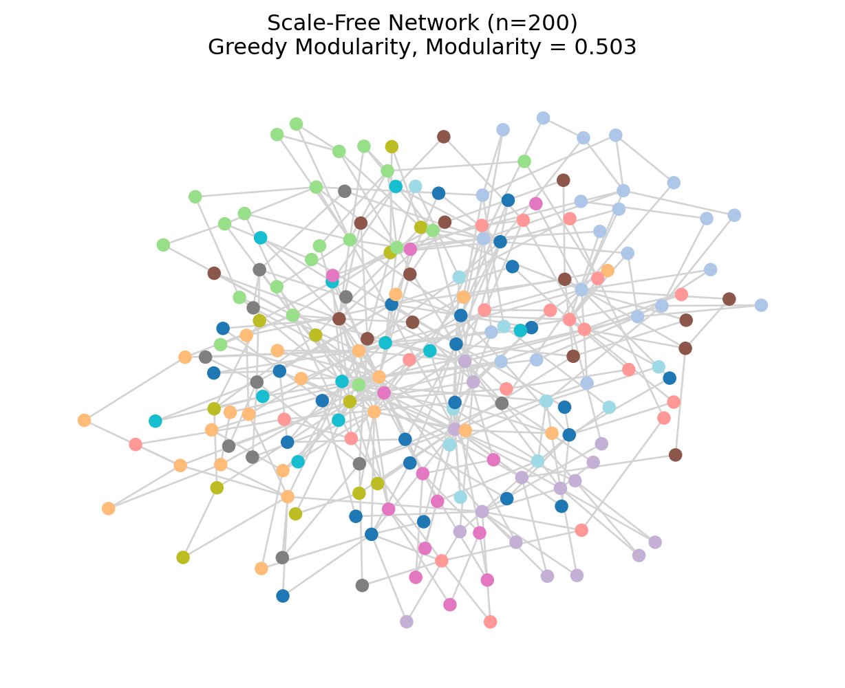

6 Key Takeaways

1. Tool Selection: NetworkX is excellent for education and small-to-medium networks. For massive graphs (millions of nodes), consider igraph or specialized tools like graph-tool.
2. Algorithm Trade-offs:
   • Greedy Modularity: Good default, deterministic.
   • Label Propagation: Fast but unstable (run it multiple times!).
   • Girvan-Newman: Great for understanding structure in small graphs, but too slow for big data.
   • Louvain: The “gold standard” for performance/quality, but requires an extra package.
3. Visual Verification: Always visualize your communities (if \(N < 1000\)) to ensure they align with the network layout.
4. Beyond Modularity: While we optimized for modularity, remember that real-world communities might overlap or have fuzzy boundaries—features that standard partition algorithms miss.

7 Exercises

1. Compare Methods on a New Network
   Load another NetworkX example graph (e.g., nx.les_miserables_graph() or nx.davis_southern_women_graph()) and:

   • Apply at least three community detection methods
   • Compare modularity scores
   • Visualize community assignments

2. Resolution Exploration (Advanced)
   Implement a simple resolution sweep for the greedy algorithm by modifying the graph (e.g., thresholding edge weights or adding/removing edges) and observe how community structure changes.

3. Community Characteristics
   For your favorite partition on the karate club graph:

   • Compute within- and between-community edge densities
   • Identify bridge nodes that connect different communities
   • Interpret what these communities might represent substantively.

---

Next Steps: After working through this Python tutorial, revisit practice_1.qmd (R) and compare the workflows and results across languages.