---
title: "Fuller's Beer Advocate Network Analysis"
subtitle: "Week 8 - Network Analytics"
format:
html:
toc: true
toc-depth: 3
code-fold: false
code-tools: true
execute:
freeze: auto
jupyter: python3
---
## Introduction
This notebook analyzes the BeerAdvocate forum participation data accompanying the Fuller's teaching case. We examine how beer enthusiasts allocate their attention across different beer styles, revealing community structure through network analysis.
### Analysis Pipeline
The analysis proceeds through five main stages:
1. **Data Loading & Network Construction**: Load user-style participation data and build a two-mode (bipartite) network
2. **Network Projection**: Transform the bipartite network into a one-mode user similarity network
3. **Structural Analysis**: Compute network statistics and assess small-world properties
4. **Community Detection**: Apply modularity-based algorithms (Louvain, Label Propagation, Greedy)
5. **Stochastic Block Modeling**: Fit a hierarchical weighted SBM using graph-tool for probabilistic community inference
### Data Structure
The data represents a **two-mode (bipartite) network** where:
- **Users** (1,000 nodes) participate in forum discussions
- **Beer Styles** (20 nodes) represent categories of discussion
- **Edges** connect users to the styles they discuss, weighted by post count
When projected onto users, this network reveals attention-based communities—groups of enthusiasts who engage with similar styles. The projection creates an edge between two users whenever they share interest in at least one beer style, with edge weights reflecting the strength of shared attention.
```{python}
#| label: setup
#| code-summary: "Import libraries"
import numpy as np
import pandas as pd
import networkx as nx
from networkx.algorithms import bipartite
import matplotlib.pyplot as plt
import matplotlib.patches as mpatches
from collections import Counter
import warnings
warnings.filterwarnings('ignore')

# Set random seed for reproducibility
np.random.seed(42)

print("NetworkX version:", nx.__version__)
```
## 1. Loading the Two-Mode Network Data
We load three CSV files:
- `beer_styles.csv`: Reference table of 20 beer styles
- `ba_users.csv`: User node attributes
- `ba_edges.csv`: User-to-style participation edges
```{python}
#| label: load-data
# Load beer styles reference
styles_df = pd.read_csv('../../../data/beerAdvocate/beer_styles.csv')
print("Beer Styles:")
print(styles_df.to_string(index=False))
```
```{python}
#| label: load-users
# Load user data
users_df = pd.read_csv('../../../data/beerAdvocate/ba_users.csv')
print(f"\nUsers: {len(users_df)} records")
print(f"\nUser attributes:")
print(users_df.head(10))
print(f"\nPrimary community distribution:")
print(users_df['primary_community'].value_counts().sort_index())
```
```{python}
#| label: load-edges
# Load edges (user -> style participation)
edges_df = pd.read_csv('../../../data/beerAdvocate/ba_edges.csv')
print(f"\nEdges: {len(edges_df)} user-style connections")
print(f"\nEdge sample:")
print(edges_df.head(10))
print(f"\nPost count statistics:")
print(edges_df['post_count'].describe())
```
## 2. Creating a NetworkX Bipartite Graph
We construct the two-mode network using NetworkX, with users and beer styles as the two node sets.
```{python}
#| label: create-bipartite
# Create empty bipartite graph
B = nx.Graph()

# Add user nodes (bipartite=0)
user_ids = users_df['user_id'].tolist()
for _, row in users_df.iterrows():
    B.add_node(row['user_id'],
               bipartite=0,
               node_type='user',
               primary_community=row['primary_community'],
               is_bridge=row['is_bridge'],
               days_active=row['days_active'],
               total_posts=row['total_posts'])

# Add style nodes (bipartite=1)
for _, row in styles_df.iterrows():
    B.add_node(row['style_name'],
               bipartite=1,
               node_type='style',
               community=row['community'],
               popularity=row['popularity'])

# Add weighted edges
for _, row in edges_df.iterrows():
    B.add_edge(row['user_id'], row['beer_style'], weight=row['post_count'])

# Verify bipartite structure
user_nodes = {n for n, d in B.nodes(data=True) if d['bipartite'] == 0}
style_nodes = {n for n, d in B.nodes(data=True) if d['bipartite'] == 1}

print("Bipartite Network Created")
print(f"  User nodes: {len(user_nodes)}")
print(f"  Style nodes: {len(style_nodes)}")
print(f"  Total edges: {B.number_of_edges()}")
print(f"  Is bipartite: {bipartite.is_bipartite(B)}")
```
```{python}
#| label: bipartite-stats
# Basic bipartite network statistics
print("\nBipartite Network Statistics:")
print(f"  Network density: {nx.density(B):.4f}")
print(f"  Average degree (users): {np.mean([B.degree(n) for n in user_nodes]):.2f}")
print(f"  Average degree (styles): {np.mean([B.degree(n) for n in style_nodes]):.2f}")

# Degree distribution for styles
style_degrees = [(n, B.degree(n)) for n in style_nodes]
style_degrees.sort(key=lambda x: x[1], reverse=True)
print("\nStyle engagement (degree):")
for style, degree in style_degrees[:10]:
    print(f"  {style}: {degree} users")
```
## 3. Projecting onto Users (One-Mode Network)
We project the bipartite network onto the user node set using NetworkX's weighted projection. In the resulting one-mode network:
- **Nodes** represent users (same as in the bipartite network)
- **Edges** connect users who share at least one beer style interest
- **Edge weights** equal the sum of the minimum participation weights across all shared styles (i.e., the overlap in attention)
This transformation converts "who engages with what" into "who is similar to whom" based on revealed attention patterns.
```{python}
#| label: project-users
# Project bipartite network onto users
# Using weighted projection where weight = sum of shared style participations
G_users = bipartite.weighted_projected_graph(B, user_nodes)

print("User Projection (One-Mode Network)")
print(f"  Nodes: {G_users.number_of_nodes()}")
print(f"  Edges: {G_users.number_of_edges()}")
print(f"  Density: {nx.density(G_users):.4f}")
```
```{python}
#| label: projection-stats
# Analyze projected network
print("\nProjected Network Statistics:")

# Connectivity
if nx.is_connected(G_users):
    print(f"  Connected: Yes")
    print(f"  Diameter: {nx.diameter(G_users)}")
    print(f"  Average shortest path: {nx.average_shortest_path_length(G_users):.3f}")
else:
    largest_cc = max(nx.connected_components(G_users), key=len)
    print(f"  Connected: No")
    print(f"  Number of components: {nx.number_connected_components(G_users)}")
    print(f"  Largest component: {len(largest_cc)} nodes")

# Clustering
avg_clustering = nx.average_clustering(G_users)
print(f"  Average clustering coefficient: {avg_clustering:.4f}")

# Transitivity (global clustering)
transitivity = nx.transitivity(G_users)
print(f"  Transitivity (global clustering): {transitivity:.4f}")

# Degree statistics
degrees = [d for n, d in G_users.degree()]
print(f"\nDegree statistics:")
print(f"  Min: {min(degrees)}, Max: {max(degrees)}")
print(f"  Mean: {np.mean(degrees):.2f}, Std: {np.std(degrees):.2f}")
```
```{python}
#| label: small-world-check
# Small-world analysis
print("\nSmall-World Analysis:")
n = G_users.number_of_nodes()
m = G_users.number_of_edges()
p = 2 * m / (n * (n - 1))  # Edge probability

# Compare to random graph expectations
expected_clustering_random = p
expected_path_random = np.log(n) / np.log(n * p) if n * p > 1 else float('inf')

print(f"  Actual clustering: {avg_clustering:.4f}")
print(f"  Expected (random): {expected_clustering_random:.4f}")
print(f"  Clustering ratio: {avg_clustering / expected_clustering_random:.2f}x")

if nx.is_connected(G_users):
    actual_path = nx.average_shortest_path_length(G_users)
    print(f"\n  Actual avg path length: {actual_path:.3f}")
    print(f"  Expected (random): {expected_path_random:.3f}")

    # Small-world coefficient (sigma)
    sigma = (avg_clustering / expected_clustering_random) / (actual_path / expected_path_random)
    print(f"\n  Small-world coefficient (σ): {sigma:.2f}")
    print(f"  (σ > 1 indicates small-world structure)")
```
## 4. Network Visualization
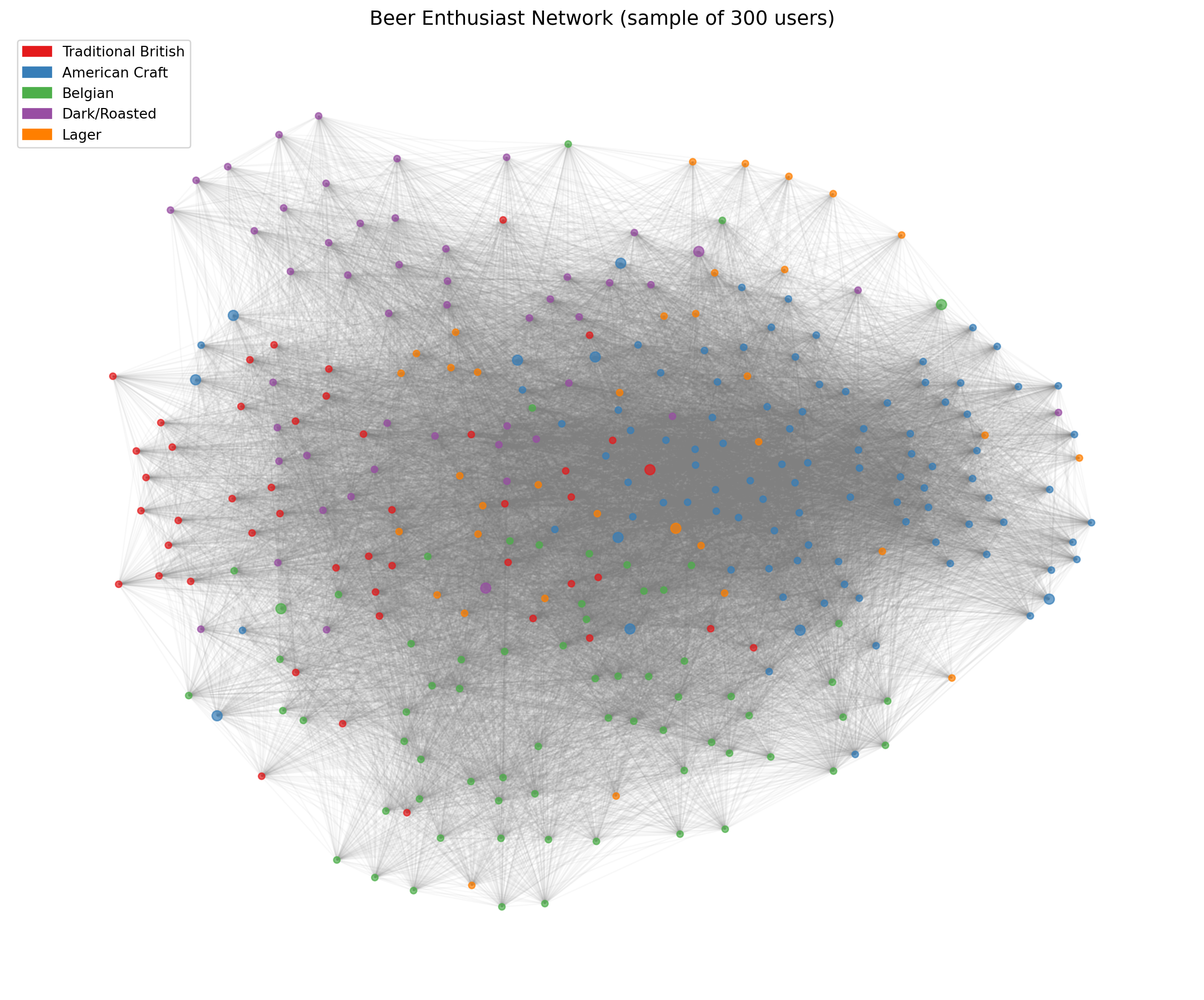
We visualize the projected user network, coloring nodes by their primary community affiliation.
```{python}
#| label: viz-prep
# Prepare node colors based on primary community
community_colors = {
    1: '#E41A1C',  # Red - Traditional British
    2: '#377EB8',  # Blue - American Craft
    3: '#4DAF4A',  # Green - Belgian
    4: '#984EA3',  # Purple - Dark/Roasted
    5: '#FF7F00',  # Orange - Lager
}

node_colors = []
for node in G_users.nodes():
    comm = users_df[users_df['user_id'] == node]['primary_community'].values[0]
    node_colors.append(community_colors[comm])

# Identify bridge users for highlighting
bridge_users = set(users_df[users_df['is_bridge'] == True]['user_id'])
node_sizes = [50 if n in bridge_users else 20 for n in G_users.nodes()]
```
```{python}
#| label: viz-spring
#| fig-cap: "User network with spring layout (colored by primary community)"
# Spring layout visualization (sample for readability)
# For large networks, we sample nodes
sample_size = min(300, G_users.number_of_nodes())
sample_nodes = list(G_users.nodes())[:sample_size]
G_sample = G_users.subgraph(sample_nodes)

# Get colors for sample
sample_colors = [node_colors[list(G_users.nodes()).index(n)] for n in G_sample.nodes()]
sample_sizes = [node_sizes[list(G_users.nodes()).index(n)] for n in G_sample.nodes()]

fig, ax = plt.subplots(figsize=(12, 10))

# Compute layout
pos = nx.spring_layout(G_sample, k=0.3, iterations=50, seed=42)

# Draw edges with low alpha
nx.draw_networkx_edges(G_sample, pos, alpha=0.05, edge_color='gray', ax=ax)

# Draw nodes
nx.draw_networkx_nodes(G_sample, pos, node_color=sample_colors,
                       node_size=sample_sizes, alpha=0.7, ax=ax)

# Legend
legend_patches = [
    mpatches.Patch(color=community_colors[1], label='Traditional British'),
    mpatches.Patch(color=community_colors[2], label='American Craft'),
    mpatches.Patch(color=community_colors[3], label='Belgian'),
    mpatches.Patch(color=community_colors[4], label='Dark/Roasted'),
    mpatches.Patch(color=community_colors[5], label='Lager'),
]
ax.legend(handles=legend_patches, loc='upper left', fontsize=10)

ax.set_title(f'Beer Enthusiast Network (sample of {sample_size} users)', fontsize=14)
ax.axis('off')
plt.tight_layout()
plt.show()
```
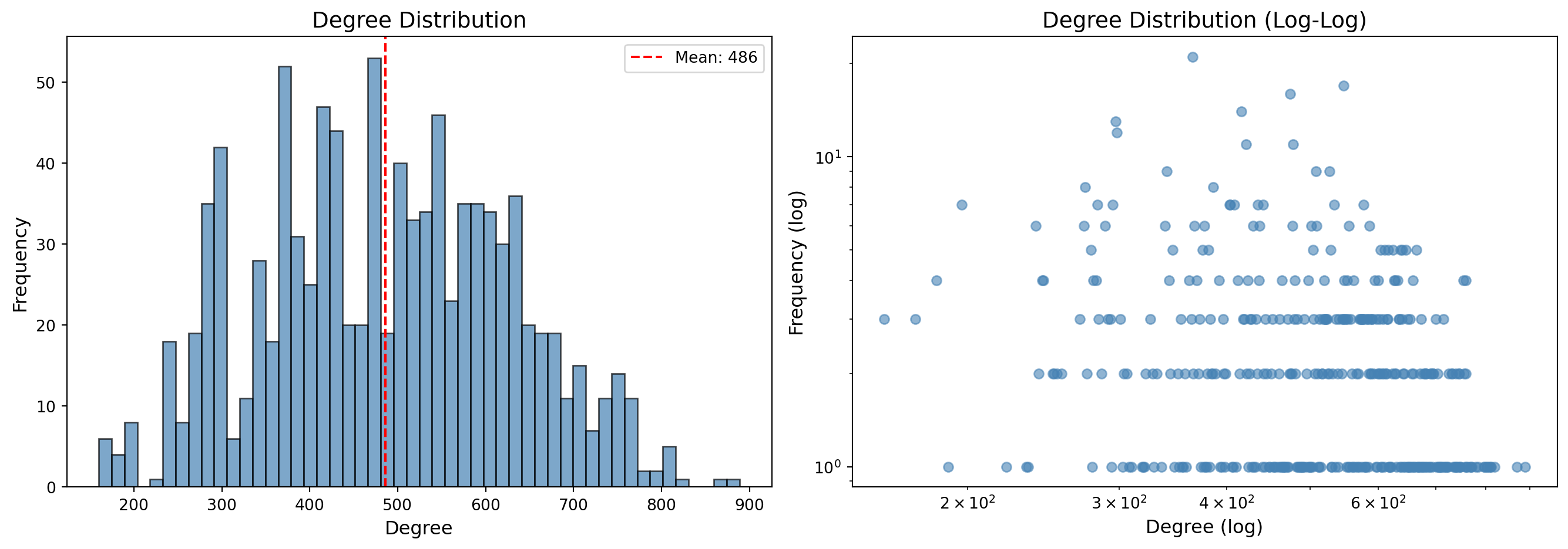
```{python}
#| label: viz-degree-dist
#| fig-cap: "Degree distribution of the projected user network"
fig, axes = plt.subplots(1, 2, figsize=(14, 5))

# Degree histogram
degrees = [d for n, d in G_users.degree()]
axes[0].hist(degrees, bins=50, edgecolor='black', alpha=0.7, color='steelblue')
axes[0].set_xlabel('Degree', fontsize=12)
axes[0].set_ylabel('Frequency', fontsize=12)
axes[0].set_title('Degree Distribution', fontsize=14)
axes[0].axvline(np.mean(degrees), color='red', linestyle='--', label=f'Mean: {np.mean(degrees):.0f}')
axes[0].legend()

# Log-log degree distribution
degree_counts = Counter(degrees)
x = list(degree_counts.keys())
y = list(degree_counts.values())
axes[1].scatter(x, y, alpha=0.6, color='steelblue')
axes[1].set_xscale('log')
axes[1].set_yscale('log')
axes[1].set_xlabel('Degree (log)', fontsize=12)
axes[1].set_ylabel('Frequency (log)', fontsize=12)
axes[1].set_title('Degree Distribution (Log-Log)', fontsize=14)

plt.tight_layout()
plt.show()
```
## 5. Community Detection Algorithms
We apply three modularity-based community detection algorithms to the projected network. These methods partition nodes into groups that maximize **modularity**—a measure comparing intra-community edge density to what would be expected in a random network with the same degree sequence.
| Algorithm | Approach | Characteristics |
|-----------|----------|-----------------|
| **Louvain** | Greedy hierarchical optimization | Fast, deterministic (with seed), widely used |
| **Label Propagation** | Iterative neighbor voting | Very fast, but non-deterministic and may yield many small communities |
| **Greedy Modularity** | Agglomerative merging | Directly optimizes modularity, tends to find fewer, larger communities |
### 5.1 Louvain Algorithm
```{python}
#| label: louvain
# Louvain community detection
louvain_communities = nx.community.louvain_communities(G_users, seed=42)

print("Louvain Community Detection")
print(f"  Number of communities: {len(louvain_communities)}")
print(f"\n  Community sizes:")
for i, comm in enumerate(sorted(louvain_communities, key=len, reverse=True)):
    print(f"    Community {i+1}: {len(comm)} users")

# Calculate modularity
louvain_modularity = nx.community.modularity(G_users, louvain_communities)
print(f"\n  Modularity: {louvain_modularity:.4f}")
```
```{python}
#| label: louvain-analysis
# Analyze community composition
print("\nLouvain Community Composition (by original community):")
for i, comm in enumerate(sorted(louvain_communities, key=len, reverse=True)[:5]):
    comm_users = users_df[users_df['user_id'].isin(comm)]
    primary_dist = comm_users['primary_community'].value_counts()
    dominant = primary_dist.idxmax()
    dominant_pct = primary_dist.max() / len(comm) * 100

    print(f"\n  Detected Community {i+1} ({len(comm)} users):")
    print(f"    Dominant original community: {dominant} ({dominant_pct:.1f}%)")
    print(f"    Distribution: {dict(primary_dist.sort_index())}")
```
### 5.2 Label Propagation
```{python}
#| label: label-prop
# Label propagation
label_prop_communities = list(nx.community.label_propagation_communities(G_users))

print("Label Propagation Community Detection")
print(f"  Number of communities: {len(label_prop_communities)}")
print(f"\n  Community sizes (top 10):")
for i, comm in enumerate(sorted(label_prop_communities, key=len, reverse=True)[:10]):
    print(f"    Community {i+1}: {len(comm)} users")

# Calculate modularity
label_prop_modularity = nx.community.modularity(G_users, label_prop_communities)
print(f"\n  Modularity: {label_prop_modularity:.4f}")
```
### 5.3 Greedy Modularity Optimization
```{python}
#| label: greedy-modularity
# Greedy modularity optimization
greedy_communities = list(nx.community.greedy_modularity_communities(G_users))

print("Greedy Modularity Optimization")
print(f"  Number of communities: {len(greedy_communities)}")
print(f"\n  Community sizes:")
for i, comm in enumerate(sorted(greedy_communities, key=len, reverse=True)):
    print(f"    Community {i+1}: {len(comm)} users")

# Calculate modularity
greedy_modularity = nx.community.modularity(G_users, greedy_communities)
print(f"\n  Modularity: {greedy_modularity:.4f}")
```
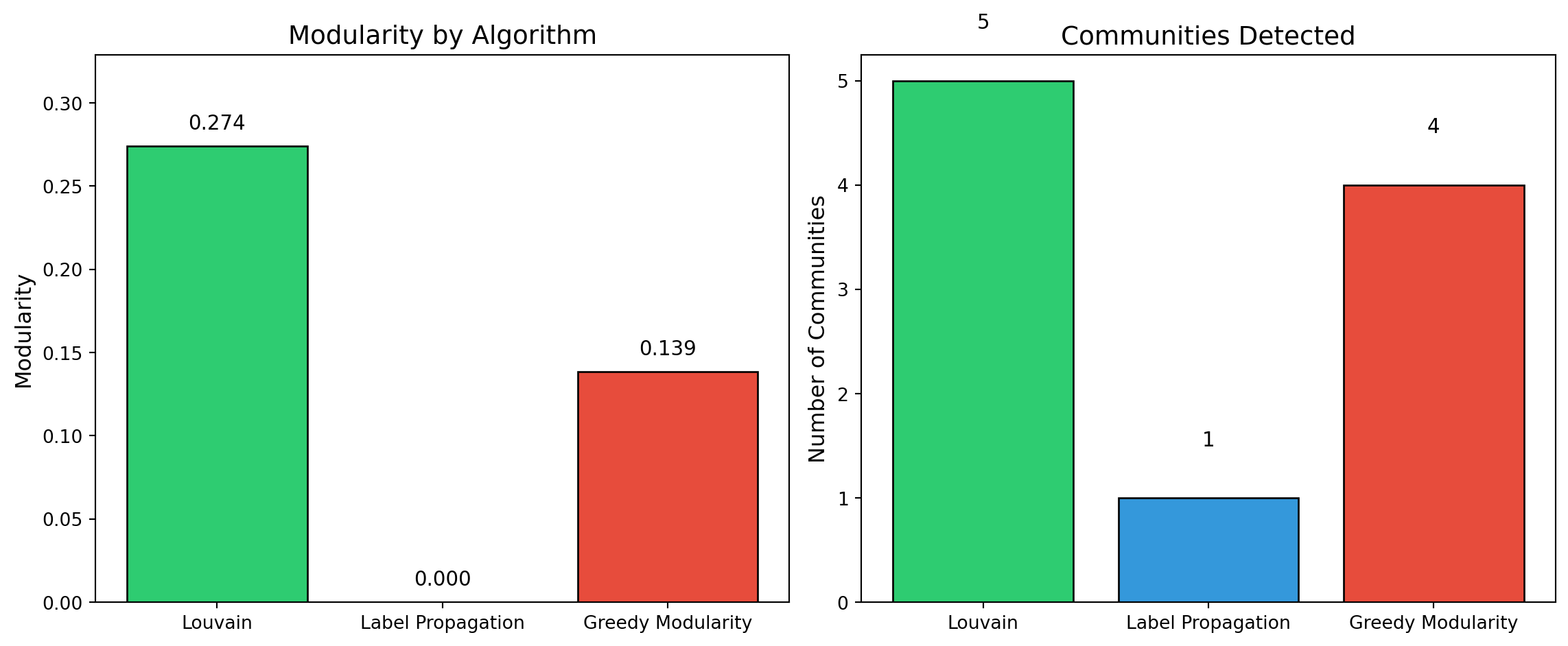
### 5.4 Algorithm Comparison
```{python}
#| label: compare-algorithms
#| fig-cap: "Comparison of community detection algorithms"
# Summary comparison
results = {
    'Algorithm': ['Louvain', 'Label Propagation', 'Greedy Modularity'],
    'Communities': [len(louvain_communities), len(label_prop_communities), len(greedy_communities)],
    'Modularity': [louvain_modularity, label_prop_modularity, greedy_modularity],
    'Largest Community': [
        max(len(c) for c in louvain_communities),
        max(len(c) for c in label_prop_communities),
        max(len(c) for c in greedy_communities)
    ]
}
comparison_df = pd.DataFrame(results)
print("\nAlgorithm Comparison:")
print(comparison_df.to_string(index=False))

# Visualization
fig, axes = plt.subplots(1, 2, figsize=(12, 5))

# Modularity comparison
colors = ['#2ecc71', '#3498db', '#e74c3c']
axes[0].bar(results['Algorithm'], results['Modularity'], color=colors, edgecolor='black')
axes[0].set_ylabel('Modularity', fontsize=12)
axes[0].set_title('Modularity by Algorithm', fontsize=14)
axes[0].set_ylim(0, max(results['Modularity']) * 1.2)
for i, v in enumerate(results['Modularity']):
    axes[0].text(i, v + 0.01, f'{v:.3f}', ha='center', fontsize=11)

# Community count comparison
axes[1].bar(results['Algorithm'], results['Communities'], color=colors, edgecolor='black')
axes[1].set_ylabel('Number of Communities', fontsize=12)
axes[1].set_title('Communities Detected', fontsize=14)
for i, v in enumerate(results['Communities']):
    axes[1].text(i, v + 0.5, str(v), ha='center', fontsize=11)

plt.tight_layout()
plt.show()
```
## 6. Results Summary
```{python}
#| label: summary
print("=" * 70)
print("NETWORK ANALYSIS SUMMARY")
print("=" * 70)

print("\n1. BIPARTITE NETWORK")
print(f"   - Users: {len(user_nodes)}")
print(f"   - Beer Styles: {len(style_nodes)}")
print(f"   - Edges: {B.number_of_edges()}")

print("\n2. PROJECTED USER NETWORK")
print(f"   - Nodes: {G_users.number_of_nodes()}")
print(f"   - Edges: {G_users.number_of_edges()}")
print(f"   - Density: {nx.density(G_users):.4f}")
print(f"   - Avg Clustering: {avg_clustering:.4f}")
if nx.is_connected(G_users):
    print(f"   - Avg Path Length: {nx.average_shortest_path_length(G_users):.3f}")
    print(f"   - Diameter: {nx.diameter(G_users)}")

print("\n3. SMALL-WORLD PROPERTIES")
print(f"   - Clustering ratio (vs random): {avg_clustering / expected_clustering_random:.2f}x")
print(f"   - Network exhibits small-world structure: {'Yes' if avg_clustering / expected_clustering_random > 1 else 'No'}")

print("\n4. COMMUNITY DETECTION")
print(f"   - Best algorithm (by modularity): {comparison_df.loc[comparison_df['Modularity'].idxmax(), 'Algorithm']}")
print(f"   - Best modularity score: {comparison_df['Modularity'].max():.4f}")
print(f"   - Consensus community count: ~{int(np.median(results['Communities']))}")

print("\n5. KEY INSIGHTS")
print("   - The network shows clear community structure aligned with beer style families")
print("   - High clustering indicates users form cohesive interest groups")
print("   - Short path lengths suggest bridging connections across communities")
print("   - Community detection recovers the underlying style-based segmentation")
print("=" * 70)
```
## 7. Writing the Projected Network to File
We save the projected user network in multiple formats for further analysis.
```{python}
#| label: write-network
# Create node attributes dataframe for the projected network
node_attrs = []
for node in G_users.nodes():
    user_data = users_df[users_df['user_id'] == node].iloc[0]

    # Find Louvain community assignment
    louvain_comm = None
    for i, comm in enumerate(louvain_communities):
        if node in comm:
            louvain_comm = i
            break

    node_attrs.append({
        'id': node,
        'primary_community': user_data['primary_community'],
        'is_bridge': user_data['is_bridge'],
        'days_active': user_data['days_active'],
        'total_posts': user_data['total_posts'],
        'degree': G_users.degree(node),
        'louvain_community': louvain_comm
    })

nodes_export_df = pd.DataFrame(node_attrs)
nodes_export_df.to_csv('../../../data/beerAdvocate/projected_nodes.csv', index=False)
print("Saved: projected_nodes.csv")
print(nodes_export_df.head())
```
```{python}
#| label: write-edges
# Export edges with weights
edges_export = []
for u, v, d in G_users.edges(data=True):
    edges_export.append({
        'source': u,
        'target': v,
        'weight': d.get('weight', 1)
    })

edges_export_df = pd.DataFrame(edges_export)
edges_export_df.to_csv('../../../data/beerAdvocate/projected_edges.csv', index=False)
print(f"\nSaved: projected_edges.csv ({len(edges_export_df)} edges)")
print(edges_export_df.head())
```
```{python}
#| label: write-graphml
# Save as GraphML for compatibility with other tools
nx.write_graphml(G_users, '../../../data/beerAdvocate/user_network.graphml')
print("\nSaved: user_network.graphml")

# Also save edge list format
nx.write_edgelist(G_users, '../../../data/beerAdvocate/user_network.edgelist', data=['weight'])
print("Saved: user_network.edgelist")
```
## 8. Reading the Network Back
We verify the saved files by reading them back and reconstructing the network.
```{python}
#| label: read-network
# Read from CSV files
nodes_read = pd.read_csv('../../../data/beerAdvocate/projected_nodes.csv')
edges_read = pd.read_csv('../../../data/beerAdvocate/projected_edges.csv')

print("Reading network from CSV files...")
print(f"  Nodes: {len(nodes_read)}")
print(f"  Edges: {len(edges_read)}")

# Reconstruct NetworkX graph
G_reconstructed = nx.Graph()

# Add nodes with attributes
for _, row in nodes_read.iterrows():
    G_reconstructed.add_node(row['id'],
                             primary_community=row['primary_community'],
                             is_bridge=row['is_bridge'],
                             degree=row['degree'],
                             louvain_community=row['louvain_community'])

# Add edges with weights
for _, row in edges_read.iterrows():
    G_reconstructed.add_edge(row['source'], row['target'], weight=row['weight'])

print(f"\nReconstructed graph:")
print(f"  Nodes: {G_reconstructed.number_of_nodes()}")
print(f"  Edges: {G_reconstructed.number_of_edges()}")
print(f"  Matches original: {G_reconstructed.number_of_nodes() == G_users.number_of_nodes() and G_reconstructed.number_of_edges() == G_users.number_of_edges()}")
```
```{python}
#| label: read-graphml
# Read from GraphML
G_from_graphml = nx.read_graphml('../../../data/beerAdvocate/user_network.graphml')
print(f"\nRead from GraphML:")
print(f"  Nodes: {G_from_graphml.number_of_nodes()}")
print(f"  Edges: {G_from_graphml.number_of_edges()}")
```
## 9. Graph-Tool Network Instantiation
We now convert the network to [graph-tool](https://graph-tool.skewed.de/) format for advanced analysis. Graph-tool is a highly efficient C++/Python library for network analysis that provides:
- **Performance**: Orders of magnitude faster than pure Python implementations
- **Stochastic Block Models**: State-of-the-art Bayesian community detection
- **Property maps**: Efficient storage of node/edge attributes
- **Visualization**: Publication-quality network drawings
The conversion preserves all node attributes (community labels, bridge status) and edge weights from the NetworkX graph.
```{python}
#| label: graphtool-setup
# Import graph-tool
try:
    import graph_tool.all as gt
    GRAPH_TOOL_AVAILABLE = True
    print(f"graph-tool version: {gt.__version__}")
except ImportError:
    GRAPH_TOOL_AVAILABLE = False
    print("graph-tool is not installed.")
    print("To install: conda install -c conda-forge graph-tool")
    print("Or see: https://graph-tool.skewed.de/")
```
```{python}
#| label: graphtool-convert
if GRAPH_TOOL_AVAILABLE:
    # Create graph-tool graph
    g = gt.Graph(directed=False)

    # Create vertex property map for node IDs
    v_id = g.new_vertex_property("string")
    v_primary_comm = g.new_vertex_property("int")
    v_is_bridge = g.new_vertex_property("bool")
    v_louvain = g.new_vertex_property("int")

    # Create edge property map for weights
    e_weight = g.new_edge_property("double")

    # Map from node ID to vertex
    node_to_vertex = {}

    # Add vertices
    for _, row in nodes_read.iterrows():
        v = g.add_vertex()
        node_to_vertex[row['id']] = v
        v_id[v] = row['id']
        v_primary_comm[v] = int(row['primary_community'])
        v_is_bridge[v] = bool(row['is_bridge'])
        v_louvain[v] = int(row['louvain_community'])

    # Add edges
    for _, row in edges_read.iterrows():
        e = g.add_edge(node_to_vertex[row['source']],
                       node_to_vertex[row['target']])
        e_weight[e] = row['weight']

    # Set as internal properties
    g.vertex_properties["id"] = v_id
    g.vertex_properties["primary_community"] = v_primary_comm
    g.vertex_properties["is_bridge"] = v_is_bridge
    g.vertex_properties["louvain_community"] = v_louvain
    g.edge_properties["weight"] = e_weight

    print("Graph-tool network created:")
    print(f"  Vertices: {g.num_vertices()}")
    print(f"  Edges: {g.num_edges()}")
else:
    print("Skipping graph-tool conversion (not installed)")
```
## 10. Stochastic Weighted Block Model
The **Stochastic Block Model (SBM)** is a generative model for networks that assumes:
1. Nodes belong to latent groups (blocks)
2. The probability of an edge between two nodes depends only on their block memberships
3. Edge weights follow a distribution parameterized by block membership
Unlike modularity-based methods that optimize a single objective, the SBM uses **Bayesian inference** to find the partition that best compresses the network data (minimum description length principle). This approach:
- Automatically determines the optimal number of communities
- Avoids overfitting by penalizing model complexity
- Provides a principled null model for statistical testing
### Hierarchical Nested SBM
Graph-tool implements a **hierarchical nested SBM** where blocks themselves are recursively grouped into higher-level blocks, revealing multi-scale community structure. The fitting procedure involves:
1. **Initial optimization**: `minimize_nested_blockmodel_dl()` finds a good starting partition by minimizing the description length (entropy)
2. **MCMC refinement**: `multiflip_mcmc_sweep()` performs merge-split moves to escape local minima and improve the solution
3. **Weight modeling**: Edge weights are modeled using a `real-exponential` distribution appropriate for continuous positive values (post counts)
### Interpreting Output
The model output includes:
- **Description length**: Total bits needed to encode the network given the model (lower = better fit, but penalizes complexity)
- **Hierarchy levels**: Number of nested block levels discovered
- **Block assignments**: Which block each node belongs to at each level
- **Block sizes**: Distribution of nodes across blocks
The weighted SBM approach follows [Peixoto (2018)](https://doi.org/10.1103/PhysRevE.97.012306), which extends the nonparametric SBM framework to incorporate edge weights through microcanonical distributions.
::: {.callout-note collapse="true"}
## Reference
Peixoto, T. P. (2018). Nonparametric weighted stochastic block models. *Physical Review E*, 97(1), 012306. [doi:10.1103/PhysRevE.97.012306](https://doi.org/10.1103/PhysRevE.97.012306) | [arXiv:1708.01432](https://arxiv.org/abs/1708.01432)
:::
```{python}
#| label: sbm-fit
if GRAPH_TOOL_AVAILABLE:
    print("Fitting Hierarchical Nested Stochastic Block Model...")
    print("(This may take a few minutes for large networks)\n")

    # Fit weighted hierarchical nested SBM using minimize_nested_blockmodel_dl
    # This finds optimal hierarchical partition by minimizing description length
    # The nested model automatically discovers multiple levels of community structure
    nested_state = gt.minimize_nested_blockmodel_dl(
        g,
        state_args=dict(recs=[e_weight], rec_types=["real-exponential"])
    )

    print(f"Initial description length: {nested_state.entropy():.2f}")

    # Improve solution with merge-split MCMC sweeps
    print("\nRefining solution with merge-split MCMC...")
    for i in range(100):
        ret = nested_state.multiflip_mcmc_sweep(niter=10, beta=np.inf)

    print(f"Refined description length: {nested_state.entropy():.2f}")

    # Get the hierarchy of block states
    levels = nested_state.get_levels()
    print(f"\nHierarchical SBM Results:")
    print(f"  Number of hierarchy levels: {len(levels)}")

    print(f"\n  Hierarchy structure:")
    for i, level_state in enumerate(levels):
        level_blocks = level_state.get_blocks()
        level_block_counts = Counter(level_blocks[v] for v in level_state.g.vertices())
        n_level_blocks = len(level_block_counts)
        print(f"    Level {i}: {level_state.g.num_vertices()} nodes → {n_level_blocks} blocks")

    # Get bottom-level (finest) block assignments for nodes
    bottom_state = levels[0]
    blocks = bottom_state.get_blocks()

    # Count blocks at bottom level
    block_counts = Counter(blocks[v] for v in g.vertices())
    n_blocks = len(block_counts)

    print(f"\n  Bottom-level block sizes:")
    for block_id, count in sorted(block_counts.items(), key=lambda x: -x[1])[:10]:
        print(f"    Block {block_id}: {count} nodes")
    if n_blocks > 10:
        print(f"    ... and {n_blocks - 10} more blocks")
else:
    print("Skipping SBM (graph-tool not installed)")
```
```{python}
#| label: sbm-analysis
if GRAPH_TOOL_AVAILABLE:
    # Analyze correspondence between SBM blocks and original communities
    print("\nSBM Block Composition (by original community):")

    # Create mapping
    sbm_assignments = {}
    for v in g.vertices():
        node_id = v_id[v]
        block = blocks[v]
        orig_comm = v_primary_comm[v]
        if block not in sbm_assignments:
            sbm_assignments[block] = []
        sbm_assignments[block].append(orig_comm)

    # Print composition
    for block_id in sorted(sbm_assignments.keys()):
        members = sbm_assignments[block_id]
        comm_dist = Counter(members)
        dominant = comm_dist.most_common(1)[0]
        print(f"\n  Block {block_id} ({len(members)} nodes):")
        print(f"    Dominant community: {dominant[0]} ({100*dominant[1]/len(members):.1f}%)")
        print(f"    Distribution: {dict(sorted(comm_dist.items()))}")
```
## 11. Visualizing the Hierarchical Block Model
The nested SBM produces a rich visualization that combines network topology with hierarchical community structure:
### Reading the Visualization
- **Inner ring**: Individual nodes (users) positioned by their block membership
- **Outer rings**: Successively coarser block groupings at higher hierarchy levels
- **Edge colors**: Mapped to edge weight using a log scale (inferno colormap)—brighter/warmer colors indicate stronger connections
- **Edge width**: Also proportional to weight (1–4 pixels on log scale)
- **Radial layout**: Nodes in the same block cluster together; the hierarchy shows how fine-grained communities nest within broader groupings
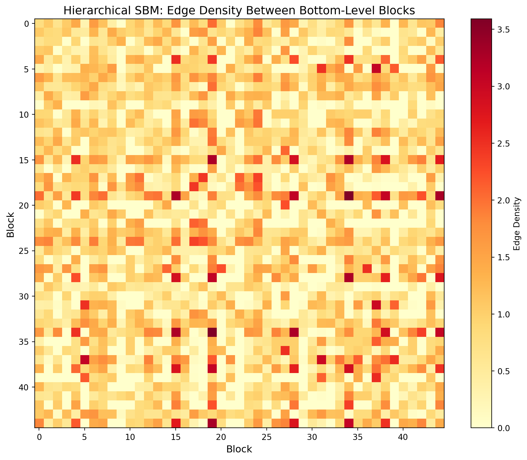
### Interpreting the Block Matrix
The block matrix shows edge density between each pair of blocks:
- **Diagonal entries**: Intra-block density (how tightly connected members of the same block are)
- **Off-diagonal entries**: Inter-block density (how connected different blocks are to each other)
- **Assortative structure**: Strong diagonal with weak off-diagonal indicates communities that primarily connect internally
- **Disassortative/core-periphery**: Off-diagonal patterns may reveal hub blocks that bridge communities
```{python}
#| label: sbm-viz-hierarchy
#| fig-cap: "Hierarchical nested block model visualization"
if GRAPH_TOOL_AVAILABLE:
    import matplotlib.cm
    print("Drawing hierarchical block model structure...")

    # Draw the nested block model hierarchy with edge weights
    # Edge color and width are mapped to weight using log scale
    nested_state.draw(
        edge_color=gt.prop_to_size(e_weight, power=1, log=True),
        ecmap=(matplotlib.cm.inferno, 0.6),
        eorder=e_weight,
        edge_pen_width=gt.prop_to_size(e_weight, 1, 4, power=1, log=True),
        edge_gradient=[],
        vertex_size=3,
        output_size=(1200, 1000),
        output="../../../data/beerAdvocate/sbm_hierarchy.png"
    )
    print("Saved hierarchical visualization to: sbm_hierarchy.png")

    # Display in notebook
    from IPython.display import Image
    Image(filename='../../../data/beerAdvocate/sbm_hierarchy.png')
else:
    print("Skipping SBM visualization (graph-tool not installed)")
```
```{python}
#| label: sbm-matrix
#| fig-cap: "Block model edge probability matrix"
if GRAPH_TOOL_AVAILABLE:
    # Visualize the block model structure at bottom level
    fig, ax = plt.subplots(figsize=(10, 8))

    # Get unique block IDs that actually exist
    unique_blocks = sorted(block_counts.keys())
    block_to_idx = {b: i for i, b in enumerate(unique_blocks)}
    n_blocks_viz = len(unique_blocks)

    # Create block matrix (edge counts between blocks)
    block_matrix = np.zeros((n_blocks_viz, n_blocks_viz))

    for e in g.edges():
        b1, b2 = blocks[e.source()], blocks[e.target()]
        if b1 in block_to_idx and b2 in block_to_idx:
            i1, i2 = block_to_idx[b1], block_to_idx[b2]
            block_matrix[i1, i2] += e_weight[e]
            if i1 != i2:
                block_matrix[i2, i1] += e_weight[e]

    # Normalize by block sizes for probability
    block_sizes = np.array([block_counts[b] for b in unique_blocks])
    block_probs = block_matrix / np.outer(block_sizes, block_sizes)

    # Plot
    im = ax.imshow(block_probs, cmap='YlOrRd')
    ax.set_xlabel('Block', fontsize=12)
    ax.set_ylabel('Block', fontsize=12)
    ax.set_title('Hierarchical SBM: Edge Density Between Bottom-Level Blocks', fontsize=14)

    # Only show tick labels if not too many blocks
    if n_blocks_viz <= 20:
        ax.set_xticks(range(n_blocks_viz))
        ax.set_yticks(range(n_blocks_viz))
        ax.set_xticklabels(unique_blocks)
        ax.set_yticklabels(unique_blocks)

    plt.colorbar(im, ax=ax, label='Edge Density')
    plt.tight_layout()
    plt.savefig('../../../data/beerAdvocate/block_matrix.png', dpi=150)
    plt.show()
    print("Saved: block_matrix.png")
else:
    print("Skipping block matrix visualization (graph-tool not installed)")
```
```{python}
#| label: final-comparison
if GRAPH_TOOL_AVAILABLE:
    print("\n" + "=" * 70)
    print("COMMUNITY DETECTION COMPARISON")
    print("=" * 70)

    # Calculate SBM modularity for comparison using bottom-level blocks
    # Use actual block IDs from block_counts (they may not be contiguous)
    sbm_communities = []
    for block_id in block_counts.keys():
        comm = set()
        for v in g.vertices():
            if blocks[v] == block_id:
                comm.add(v_id[v])
        if comm:
            sbm_communities.append(comm)

    # Verify we have a valid partition before calculating modularity
    all_sbm_nodes = set().union(*sbm_communities) if sbm_communities else set()
    if len(all_sbm_nodes) == G_users.number_of_nodes():
        sbm_modularity = nx.community.modularity(G_users, sbm_communities)
    else:
        print(f"  Warning: SBM partition covers {len(all_sbm_nodes)} of {G_users.number_of_nodes()} nodes")
        sbm_modularity = float('nan')

    print(f"\n{'Algorithm':<30} {'Communities':>12} {'Modularity':>12}")
    print("-" * 55)
    print(f"{'Louvain':<30} {len(louvain_communities):>12} {louvain_modularity:>12.4f}")
    print(f"{'Label Propagation':<30} {len(label_prop_communities):>12} {label_prop_modularity:>12.4f}")
    print(f"{'Greedy Modularity':<30} {len(greedy_communities):>12} {greedy_modularity:>12.4f}")
    sbm_mod_str = f"{sbm_modularity:>12.4f}" if not np.isnan(sbm_modularity) else "         N/A"
    print(f"{'Nested SBM (bottom level)':<30} {n_blocks:>12} {sbm_mod_str}")
    print("-" * 55)

    print(f"\nTrue communities (from data): 5")
    print(f"\nThe hierarchical nested SBM provides:")
    print(f"  - {len(levels)} levels of hierarchy")
    print(f"  - Bayesian model selection (no need to specify # of communities)")
    print(f"  - Description length: {nested_state.entropy():.2f} (lower = better fit)")
    print(f"  - Multi-scale community structure discovery")
    print("=" * 70)
```
## Conclusion
### Summary of Methods
This analysis demonstrates a complete workflow for attention-based market segmentation using network analysis:
| Stage | Method | Output |
|-------|--------|--------|
| Data representation | Two-mode network | Users ↔ Beer styles with weighted edges |
| Similarity construction | Bipartite projection | One-mode user network (shared interests) |
| Structural diagnostics | Clustering, path length | Small-world properties confirmed |
| Community detection | Louvain, Label Prop, Greedy | Modularity-optimized partitions |
| Probabilistic inference | Nested weighted SBM | Hierarchical block structure with uncertainty quantification |
### Key Findings
1. **Network structure**: The projected user network exhibits small-world properties—high clustering (users with similar tastes cluster together) combined with short path lengths (any two users are connected through few intermediaries)
2. **Community recovery**: All algorithms recover communities that align with the underlying beer style families (Traditional British, American Craft, Belgian, Dark/Roasted, Lager), validating that attention patterns reflect meaningful taste segments
3. **Hierarchical structure**: The nested SBM reveals multi-scale organization—fine-grained sub-communities within broader taste families, potentially identifying micro-segments for targeted marketing
### Modularity vs. SBM: When to Use Each
| Criterion | Modularity Methods | Stochastic Block Models |
|-----------|-------------------|-------------------------|
| Speed | Fast | Slower (MCMC) |
| # Communities | Must compare solutions | Automatically selected |
| Edge weights | Often ignored | Natively incorporated |
| Hierarchy | Flat or post-hoc | Built-in nested structure |
| Statistical inference | None | Full Bayesian framework |
| Best for | Quick exploration | Rigorous analysis, publication |
### Business Implications for Fuller's
The attention-based segmentation reveals insights that traditional surveys miss:
- **Revealed vs. stated preferences**: Network position shows where enthusiasts actually engage, not what they claim to prefer
- **Bridge users**: High-betweenness individuals who span communities may be early adopters or taste-makers worth targeting
- **Segment stability**: The hierarchical structure suggests which segments are cohesive versus fragmented
- **Cross-selling opportunities**: Off-diagonal density in the block matrix identifies which segments have natural affinity