quarterly_metrics |>
  pivot_longer(
    cols = matches("^(revenue|cost)_Q[1-4]$"),
    names_to = c(".value", "quarter"),
    names_pattern = "(revenue|cost)_(Q[1-4])",
    values_transform = list(revenue = as.double, cost = as.double)
)Pivoting Data: Wide ↔︎ Long Transformations
The Art of Data Reshaping 🔄
Data pivoting is the cornerstone of data tidying - the ability to transform data between wide and long formats. Think of it as rotating your data table to change its perspective. Wide format spreads variables across columns (good for human reading), while long format stacks data into rows (ideal for analysis and visualization).
Specify the column-name contract
When names encode several variables, describe the pattern explicitly. The special .value sentinel tells pivot_longer() that part of each source name should become an output value column:
For a column called revenue_Q2, the regular expression captures revenue as the output value-column name and Q2 as the quarter. values_transform enforces numeric types during the pivot. Columns that do not match are excluded deliberately, which prevents an identifier from being reshaped accidentally.
Understanding Wide vs. Long Format
Let’s start with a clear comparison:
library(tidyverse)
library(lubridate)

# Wide format: Values spread across columns
sales_wide <- tibble(
  quarter = c("Q1", "Q2", "Q3", "Q4"),
  north = c(150000, 162000, 158000, 175000),
  south = c(142000, 155000, 168000, 180000),
  east = c(138000, 148000, 152000, 165000),
  west = c(145000, 158000, 163000, 172000)
)

cat("WIDE FORMAT: Each region is a separate column\n")
WIDE FORMAT: Each region is a separate columnprint(sales_wide)# A tibble: 4 × 5
quarter north south east west
<chr> <dbl> <dbl> <dbl> <dbl>
1 Q1 150000 142000 138000 145000
2 Q2 162000 155000 148000 158000
3 Q3 158000 168000 152000 163000
4 Q4 175000 180000 165000 172000# Long format: Values stacked in rows
sales_long <- sales_wide %>%
pivot_longer(
cols = c(north, south, east, west),
names_to = "region",
values_to = "sales"
)
cat("\nLONG FORMAT: All sales values in one column\n")
LONG FORMAT: All sales values in one columnprint(sales_long)# A tibble: 16 × 3
quarter region sales
<chr> <chr> <dbl>
1 Q1 north 150000
2 Q1 south 142000
3 Q1 east 138000
4 Q1 west 145000
5 Q2 north 162000
6 Q2 south 155000
7 Q2 east 148000
8 Q2 west 158000
9 Q3 north 158000
10 Q3 south 168000
11 Q3 east 152000
12 Q3 west 163000
13 Q4 north 175000
14 Q4 south 180000
15 Q4 east 165000
16 Q4 west 172000cat("\nComparison:\n")
Comparison:cat("Wide: ", nrow(sales_wide), " rows x ", ncol(sales_wide), " columns\n")Wide: 4 rows x 5 columnscat("Long: ", nrow(sales_long), " rows x ", ncol(sales_long), " columns\n")Long: 16 rows x 3 columnsWhen to Use Each Format
cat("📊 WIDE FORMAT - Best for:\n")📊 WIDE FORMAT - Best for:cat("- Human-readable reports and dashboards\n")- Human-readable reports and dashboardscat("- Side-by-side comparisons\n")- Side-by-side comparisonscat("- Spreadsheet-style presentations\n")- Spreadsheet-style presentationscat("- Correlation matrices\n")- Correlation matricescat("- Crosstabs and pivot tables\n\n")- Crosstabs and pivot tablescat("📈 LONG FORMAT - Best for:\n")📈 LONG FORMAT - Best for:cat("- ggplot2 visualizations\n")- ggplot2 visualizationscat("- Statistical modeling and analysis\n")- Statistical modeling and analysiscat("- Group-by operations with dplyr\n")- Group-by operations with dplyrcat("- Time series analysis\n")- Time series analysiscat("- Machine learning datasets\n\n")- Machine learning datasets# Demonstrate why ggplot2 prefers long format
library(ggplot2)
# This works beautifully with long format
sales_long %>%
ggplot(aes(x = quarter, y = sales, color = region, group = region)) +
geom_line(size = 1.2) +
geom_point(size = 3) +
scale_y_continuous(labels = scales::dollar_format(scale = 1e-3, suffix = "K")) +
labs(
title = "Regional Sales Performance by Quarter",
subtitle = "Long format makes this visualization straightforward",
x = "Quarter",
y = "Sales ($)",
color = "Region"
) +
theme_minimal()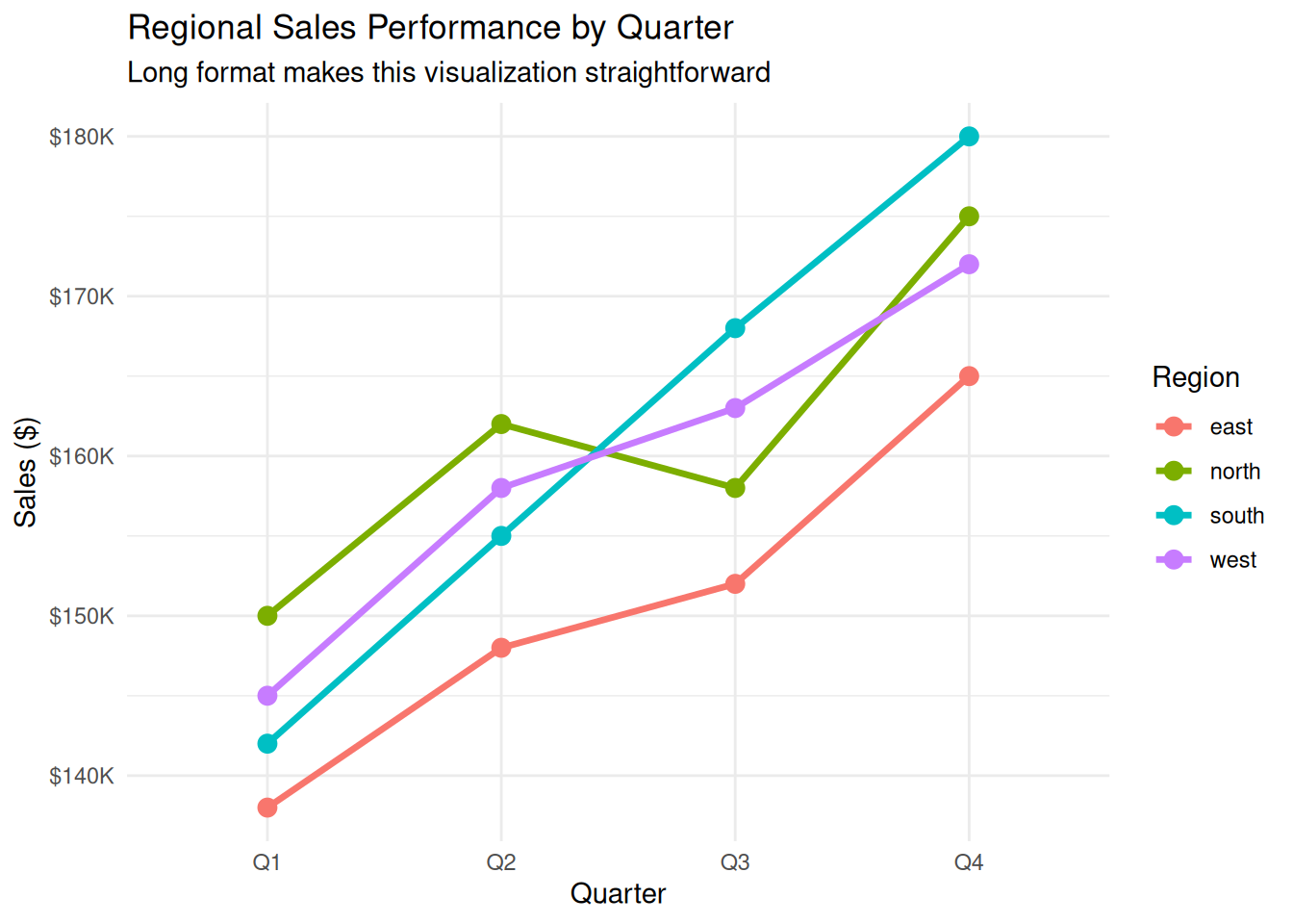
pivot_longer(): Wide to Long
pivot_longer() transforms wide data to long format by “gathering” multiple columns into key-value pairs.
Basic Syntax and Common Patterns
# Real-world example: Employee performance ratings
performance_wide <- tibble(
  employee_id = 1:5,
  name = c("Alice Johnson", "Bob Smith", "Carol Davis", "David Wilson", "Emma Brown"),
  department = c("Sales", "Marketing", "IT", "Sales", "Marketing"),
  communication_q1 = c(4.2, 3.8, 4.5, 3.9, 4.1),
  communication_q2 = c(4.3, 4.0, 4.6, 4.1, 4.2),
  teamwork_q1 = c(4.0, 4.2, 4.3, 3.8, 4.4),
  teamwork_q2 = c(4.1, 4.4, 4.4, 4.0, 4.6),
  leadership_q1 = c(3.8, 3.5, 4.1, 3.6, 3.9),
  leadership_q2 = c(4.0, 3.7, 4.3, 3.8, 4.1)
)

cat("Original wide format (multiple rating columns):\n")
Original wide format (multiple rating columns):print(performance_wide)# A tibble: 5 × 9
employee_id name department communication_q1 communication_q2 teamwork_q1
<int> <chr> <chr> <dbl> <dbl> <dbl>
1 1 Alice Jo… Sales 4.2 4.3 4
2 2 Bob Smith Marketing 3.8 4 4.2
3 3 Carol Da… IT 4.5 4.6 4.3
4 4 David Wi… Sales 3.9 4.1 3.8
5 5 Emma Bro… Marketing 4.1 4.2 4.4
# ℹ 3 more variables: teamwork_q2 <dbl>, leadership_q1 <dbl>,
# leadership_q2 <dbl># Method 1: Basic pivot_longer
performance_long_basic <- performance_wide %>%
pivot_longer(
cols = communication_q1:leadership_q2, # Columns to pivot
names_to = "skill_quarter", # Name for the new key column
values_to = "rating" # Name for the new value column
)
cat("\nBasic pivot_longer result:\n")
Basic pivot_longer result:print(head(performance_long_basic, 10))# A tibble: 10 × 5
employee_id name department skill_quarter rating
<int> <chr> <chr> <chr> <dbl>
1 1 Alice Johnson Sales communication_q1 4.2
2 1 Alice Johnson Sales communication_q2 4.3
3 1 Alice Johnson Sales teamwork_q1 4
4 1 Alice Johnson Sales teamwork_q2 4.1
5 1 Alice Johnson Sales leadership_q1 3.8
6 1 Alice Johnson Sales leadership_q2 4
7 2 Bob Smith Marketing communication_q1 3.8
8 2 Bob Smith Marketing communication_q2 4
9 2 Bob Smith Marketing teamwork_q1 4.2
10 2 Bob Smith Marketing teamwork_q2 4.4Advanced Column Selection
# Method 2: Using column selection helpers
performance_long_helpers <- performance_wide %>%
  pivot_longer(
    cols = contains("_q"),               # All columns containing "_q"
    names_to = "skill_quarter",
    values_to = "rating"
  )

# Method 3: Excluding specific columns
performance_long_exclude <- performance_wide %>%
  pivot_longer(
    cols = -c(employee_id, name, department),  # Everything except these
    names_to = "skill_quarter",
    values_to = "rating"
  )

# Method 4: Using patterns with matches()
performance_long_pattern <- performance_wide %>%
  pivot_longer(
    cols = matches("(communication|teamwork|leadership)_q[12]"),  # Regex pattern
    names_to = "skill_quarter",
    values_to = "rating"
  )

cat("All methods produce identical results:\n")
All methods produce identical results:cat("Basic: ", nrow(performance_long_basic), " rows\n")Basic: 30 rowscat("Helpers: ", nrow(performance_long_helpers), " rows\n")Helpers: 30 rowscat("Exclude: ", nrow(performance_long_exclude), " rows\n")Exclude: 30 rowscat("Pattern: ", nrow(performance_long_pattern), " rows\n")Pattern: 30 rowsSeparating Column Names
The real power comes when you separate the pivoted column names:
# Separate skill and quarter into different columns
performance_tidy <- performance_wide %>%
  pivot_longer(
    cols = contains("_q"),
    names_to = "skill_quarter",
    values_to = "rating"
  ) %>%
  separate(
    skill_quarter,
    into = c("skill", "quarter"),
    sep = "_"
  ) %>%
  mutate(
    quarter = str_replace(quarter, "q", "Q"),  # Clean up quarter format
    quarter_num = as.numeric(str_extract(quarter, "\\d+")),
    skill = str_to_title(skill)
  )

cat("Cleaned and separated data:\n")
Cleaned and separated data:print(head(performance_tidy, 12))# A tibble: 12 × 7
employee_id name department skill quarter rating quarter_num
<int> <chr> <chr> <chr> <chr> <dbl> <dbl>
1 1 Alice Johnson Sales Communication Q1 4.2 1
2 1 Alice Johnson Sales Communication Q2 4.3 2
3 1 Alice Johnson Sales Teamwork Q1 4 1
4 1 Alice Johnson Sales Teamwork Q2 4.1 2
5 1 Alice Johnson Sales Leadership Q1 3.8 1
6 1 Alice Johnson Sales Leadership Q2 4 2
7 2 Bob Smith Marketing Communication Q1 3.8 1
8 2 Bob Smith Marketing Communication Q2 4 2
9 2 Bob Smith Marketing Teamwork Q1 4.2 1
10 2 Bob Smith Marketing Teamwork Q2 4.4 2
11 2 Bob Smith Marketing Leadership Q1 3.5 1
12 2 Bob Smith Marketing Leadership Q2 3.7 2# Now analysis becomes powerful
cat("\nAverage ratings by skill and quarter:\n")
Average ratings by skill and quarter:performance_tidy %>%
group_by(skill, quarter) %>%
summarise(
avg_rating = round(mean(rating), 2),
employees = n(),
.groups = "drop"
) %>%
pivot_wider(names_from = quarter, values_from = avg_rating) %>%
print()# A tibble: 3 × 4
skill employees Q1 Q2
<chr> <int> <dbl> <dbl>
1 Communication 5 4.1 4.24
2 Leadership 5 3.78 3.98
3 Teamwork 5 4.14 4.3 Handling Multiple Value Columns
# Complex example: Survey with both scores and confidence levels
survey_complex <- tibble(
  participant_id = 1:4,
  age_group = c("18-25", "26-35", "36-45", "46-55"),
  satisfaction_score_pre = c(3.2, 4.1, 2.8, 3.9),
  satisfaction_confidence_pre = c(0.8, 0.9, 0.7, 0.85),
  satisfaction_score_post = c(4.1, 4.5, 3.9, 4.2),
  satisfaction_confidence_post = c(0.9, 0.95, 0.85, 0.9),
  recommendation_score_pre = c(2.8, 3.5, 2.1, 3.2),
  recommendation_confidence_pre = c(0.7, 0.8, 0.6, 0.75),
  recommendation_score_post = c(3.9, 4.2, 3.4, 4.0),
  recommendation_confidence_post = c(0.85, 0.9, 0.8, 0.88)
)

cat("Complex survey data with scores and confidence:\n")
Complex survey data with scores and confidence:print(survey_complex)# A tibble: 4 × 10
participant_id age_group satisfaction_score_pre satisfaction_confidence_pre
<int> <chr> <dbl> <dbl>
1 1 18-25 3.2 0.8
2 2 26-35 4.1 0.9
3 3 36-45 2.8 0.7
4 4 46-55 3.9 0.85
# ℹ 6 more variables: satisfaction_score_post <dbl>,
# satisfaction_confidence_post <dbl>, recommendation_score_pre <dbl>,
# recommendation_confidence_pre <dbl>, recommendation_score_post <dbl>,
# recommendation_confidence_post <dbl># Pivot multiple value types simultaneously
survey_long <- survey_complex %>%
pivot_longer(
cols = -c(participant_id, age_group),
names_to = c("metric", "measure", "period"),
names_pattern = "(.+)_(score|confidence)_(pre|post)",
values_to = "value"
) %>%
pivot_wider(
names_from = measure,
values_from = value
) %>%
mutate(
metric = str_to_title(metric),
period = str_to_title(period)
)
cat("\nTransformed to tidy format with separate score/confidence columns:\n")
Transformed to tidy format with separate score/confidence columns:print(head(survey_long, 10))# A tibble: 10 × 6
participant_id age_group metric period score confidence
<int> <chr> <chr> <chr> <dbl> <dbl>
1 1 18-25 Satisfaction Pre 3.2 0.8
2 1 18-25 Satisfaction Post 4.1 0.9
3 1 18-25 Recommendation Pre 2.8 0.7
4 1 18-25 Recommendation Post 3.9 0.85
5 2 26-35 Satisfaction Pre 4.1 0.9
6 2 26-35 Satisfaction Post 4.5 0.95
7 2 26-35 Recommendation Pre 3.5 0.8
8 2 26-35 Recommendation Post 4.2 0.9
9 3 36-45 Satisfaction Pre 2.8 0.7
10 3 36-45 Satisfaction Post 3.9 0.85# Calculate improvement with confidence intervals
improvements <- survey_long %>%
select(-age_group) %>%
pivot_wider(names_from = period, values_from = c(score, confidence)) %>%
mutate(
score_improvement = score_Post - score_Pre,
confidence_avg = (confidence_Pre + confidence_Post) / 2,
improvement_category = case_when(
score_improvement >= 1.0 ~ "Significant Improvement",
score_improvement >= 0.5 ~ "Moderate Improvement",
score_improvement >= 0.0 ~ "Slight Improvement",
TRUE ~ "Decline"
)
)
cat("\nImprovement analysis:\n")
Improvement analysis:improvements %>%
group_by(metric, improvement_category) %>%
summarise(
participants = n(),
avg_improvement = round(mean(score_improvement), 2),
avg_confidence = round(mean(confidence_avg), 2),
.groups = "drop"
) %>%
arrange(metric, desc(avg_improvement)) %>%
print()# A tibble: 5 × 5
metric improvement_category participants avg_improvement avg_confidence
<chr> <chr> <int> <dbl> <dbl>
1 Recommendati… Significant Improve… 2 1.2 0.74
2 Recommendati… Moderate Improvement 2 0.75 0.83
3 Satisfaction Significant Improve… 1 1.1 0.77
4 Satisfaction Moderate Improvement 1 0.9 0.85
5 Satisfaction Slight Improvement 2 0.35 0.9 pivot_wider(): Long to Wide
pivot_wider() spreads key-value pairs into separate columns, creating the inverse of pivot_longer().
Basic Wide Transformation
# Start with our long performance data
cat("Starting with long format data:\n")
Starting with long format data:print(head(performance_tidy, 8))# A tibble: 8 × 7
employee_id name department skill quarter rating quarter_num
<int> <chr> <chr> <chr> <chr> <dbl> <dbl>
1 1 Alice Johnson Sales Communication Q1 4.2 1
2 1 Alice Johnson Sales Communication Q2 4.3 2
3 1 Alice Johnson Sales Teamwork Q1 4 1
4 1 Alice Johnson Sales Teamwork Q2 4.1 2
5 1 Alice Johnson Sales Leadership Q1 3.8 1
6 1 Alice Johnson Sales Leadership Q2 4 2
7 2 Bob Smith Marketing Communication Q1 3.8 1
8 2 Bob Smith Marketing Communication Q2 4 2# Convert back to wide format for reporting
performance_report <- performance_tidy %>%
# Create quarter-skill combinations
unite("quarter_skill", quarter, skill, sep = "_") %>%
pivot_wider(
names_from = quarter_skill,
values_from = rating
) %>%
arrange(department, name)
cat("\nConverted to wide format for reporting:\n")
Converted to wide format for reporting:print(performance_report)# A tibble: 10 × 10
employee_id name department quarter_num Q1_Communication Q2_Communication
<int> <chr> <chr> <dbl> <dbl> <dbl>
1 3 Carol D… IT 1 4.5 NA
2 3 Carol D… IT 2 NA 4.6
3 2 Bob Smi… Marketing 1 3.8 NA
4 2 Bob Smi… Marketing 2 NA 4
5 5 Emma Br… Marketing 1 4.1 NA
6 5 Emma Br… Marketing 2 NA 4.2
7 1 Alice J… Sales 1 4.2 NA
8 1 Alice J… Sales 2 NA 4.3
9 4 David W… Sales 1 3.9 NA
10 4 David W… Sales 2 NA 4.1
# ℹ 4 more variables: Q1_Teamwork <dbl>, Q2_Teamwork <dbl>,
# Q1_Leadership <dbl>, Q2_Leadership <dbl>Business Intelligence Dashboard Format
# Create dashboard-ready format
dashboard_data <- performance_tidy %>%
  group_by(employee_id, name, department, quarter) %>%
  summarise(
    avg_rating = round(mean(rating), 2),
    skills_evaluated = n(),
    .groups = "drop"
  ) %>%
  pivot_wider(
    names_from = quarter,
    values_from = c(avg_rating, skills_evaluated),
    names_sep = "_"
  ) %>%
  # Calculate improvements
  mutate(
    improvement_q1_to_q2 = round(avg_rating_Q2 - avg_rating_Q1, 2),
    improvement_category = case_when(
      improvement_q1_to_q2 >= 0.3 ~ "Strong Growth",
      improvement_q1_to_q2 >= 0.1 ~ "Steady Growth",
      improvement_q1_to_q2 >= -0.1 ~ "Stable",
      TRUE ~ "Needs Attention"
    )
  )

cat("Dashboard-ready format:\n")
Dashboard-ready format:print(dashboard_data)# A tibble: 5 × 9
employee_id name department avg_rating_Q1 avg_rating_Q2 skills_evaluated_Q1
<int> <chr> <chr> <dbl> <dbl> <int>
1 1 Alice … Sales 4 4.13 3
2 2 Bob Sm… Marketing 3.83 4.03 3
3 3 Carol … IT 4.3 4.43 3
4 4 David … Sales 3.77 3.97 3
5 5 Emma B… Marketing 4.13 4.3 3
# ℹ 3 more variables: skills_evaluated_Q2 <int>, improvement_q1_to_q2 <dbl>,
# improvement_category <chr># Summary by department
cat("\nDepartment performance summary:\n")
Department performance summary:dashboard_data %>%
group_by(department) %>%
summarise(
employees = n(),
avg_q1_rating = round(mean(avg_rating_Q1), 2),
avg_q2_rating = round(mean(avg_rating_Q2), 2),
avg_improvement = round(mean(improvement_q1_to_q2), 2),
strong_growth_pct = round(100 * mean(improvement_category == "Strong Growth"), 1),
.groups = "drop"
) %>%
arrange(desc(avg_improvement)) %>%
print()# A tibble: 3 × 6
department employees avg_q1_rating avg_q2_rating avg_improvement
<chr> <int> <dbl> <dbl> <dbl>
1 Marketing 2 3.98 4.16 0.18
2 Sales 2 3.88 4.05 0.16
3 IT 1 4.3 4.43 0.13
# ℹ 1 more variable: strong_growth_pct <dbl>Handling Missing Values in Pivoting
# Realistic scenario with missing data
incomplete_sales <- tibble(
  month = rep(c("Jan", "Feb", "Mar"), each = 3),
  region = rep(c("North", "South", "West"), 3),
  sales = c(100, 150, NA, 120, NA, 180, 130, 160, 170)
)

cat("Data with missing values:\n")
Data with missing values:print(incomplete_sales)# A tibble: 9 × 3
month region sales
<chr> <chr> <dbl>
1 Jan North 100
2 Jan South 150
3 Jan West NA
4 Feb North 120
5 Feb South NA
6 Feb West 180
7 Mar North 130
8 Mar South 160
9 Mar West 170# Pivot wider with missing values
sales_matrix <- incomplete_sales %>%
pivot_wider(
names_from = month,
values_from = sales,
values_fill = 0 # Fill missing with 0 for this business case
)
cat("\nPivoted wide with missing values filled as 0:\n")
Pivoted wide with missing values filled as 0:print(sales_matrix)# A tibble: 3 × 4
region Jan Feb Mar
<chr> <dbl> <dbl> <dbl>
1 North 100 120 130
2 South 150 NA 160
3 West NA 180 170# Alternative: Keep NAs and handle explicitly
sales_matrix_na <- incomplete_sales %>%
pivot_wider(
names_from = month,
values_from = sales
# No values_fill - keeps NAs
) %>%
mutate(
total_known = rowSums(select(., Jan:Mar), na.rm = TRUE),
months_reported = rowSums(!is.na(select(., Jan:Mar))),
avg_monthly = round(total_known / months_reported, 1)
)
cat("\nWith explicit missing value handling:\n")
With explicit missing value handling:print(sales_matrix_na)# A tibble: 3 × 7
region Jan Feb Mar total_known months_reported avg_monthly
<chr> <dbl> <dbl> <dbl> <dbl> <dbl> <dbl>
1 North 100 120 130 350 3 117.
2 South 150 NA 160 310 2 155
3 West NA 180 170 350 2 175 Complex Real-World Scenarios
Financial Data Transformation
# Quarterly financial statements across multiple companies
financials_raw <- tibble(
  company = rep(c("TechCorp", "RetailCo", "ManufactureInc"), each = 4),
  metric = rep(c("revenue", "costs", "profit", "employees"), 3),
  q1_2023 = c(
    # TechCorp
    5200, 3800, 1400, 450,
    # RetailCo
    8900, 7100, 1800, 1200,
    # ManufactureInc
    6700, 5200, 1500, 800
  ),
  q2_2023 = c(
    5800, 4100, 1700, 470,
    9200, 7300, 1900, 1250,
    7100, 5500, 1600, 820
  ),
  q3_2023 = c(
    6100, 4200, 1900, 485,
    9800, 7600, 2200, 1300,
    7400, 5800, 1600, 835
  ),
  q4_2023 = c(
    6500, 4400, 2100, 500,
    10200, 7900, 2300, 1320,
    7800, 6100, 1700, 850
  )
)

cat("Raw financial data (wide format):\n")
Raw financial data (wide format):print(head(financials_raw, 12))# A tibble: 12 × 6
company metric q1_2023 q2_2023 q3_2023 q4_2023
<chr> <chr> <dbl> <dbl> <dbl> <dbl>
1 TechCorp revenue 5200 5800 6100 6500
2 TechCorp costs 3800 4100 4200 4400
3 TechCorp profit 1400 1700 1900 2100
4 TechCorp employees 450 470 485 500
5 RetailCo revenue 8900 9200 9800 10200
6 RetailCo costs 7100 7300 7600 7900
7 RetailCo profit 1800 1900 2200 2300
8 RetailCo employees 1200 1250 1300 1320
9 ManufactureInc revenue 6700 7100 7400 7800
10 ManufactureInc costs 5200 5500 5800 6100
11 ManufactureInc profit 1500 1600 1600 1700
12 ManufactureInc employees 800 820 835 850# Transform to analysis-ready format
financials_clean <- financials_raw %>%
# First pivot to long format
pivot_longer(
cols = starts_with("q"),
names_to = "quarter",
values_to = "value"
) %>%
# Then pivot wider to separate metrics
pivot_wider(
names_from = metric,
values_from = value
) %>%
# Clean and enhance
mutate(
quarter = str_replace(quarter, "q(\\d)_", "Q\\1 "),
profit_margin = round(profit / revenue * 100, 1),
revenue_per_employee = round(revenue / employees * 1000, 0),
cost_efficiency = round(costs / revenue * 100, 1)
) %>%
arrange(company, quarter)
cat("\nCleaned financial analysis format:\n")
Cleaned financial analysis format:print(head(financials_clean, 9))# A tibble: 9 × 9
company quarter revenue costs profit employees profit_margin
<chr> <chr> <dbl> <dbl> <dbl> <dbl> <dbl>
1 ManufactureInc Q1 2023 6700 5200 1500 800 22.4
2 ManufactureInc Q2 2023 7100 5500 1600 820 22.5
3 ManufactureInc Q3 2023 7400 5800 1600 835 21.6
4 ManufactureInc Q4 2023 7800 6100 1700 850 21.8
5 RetailCo Q1 2023 8900 7100 1800 1200 20.2
6 RetailCo Q2 2023 9200 7300 1900 1250 20.7
7 RetailCo Q3 2023 9800 7600 2200 1300 22.4
8 RetailCo Q4 2023 10200 7900 2300 1320 22.5
9 TechCorp Q1 2023 5200 3800 1400 450 26.9
# ℹ 2 more variables: revenue_per_employee <dbl>, cost_efficiency <dbl># Performance analysis
cat("\nCompany performance comparison:\n")
Company performance comparison:financials_clean %>%
group_by(company) %>%
summarise(
avg_profit_margin = round(mean(profit_margin), 1),
revenue_growth = round((last(revenue) - first(revenue)) / first(revenue) * 100, 1),
avg_revenue_per_employee = round(mean(revenue_per_employee), 0),
cost_trend = round(last(cost_efficiency) - first(cost_efficiency), 1),
.groups = "drop"
) %>%
arrange(desc(avg_profit_margin)) %>%
print()# A tibble: 3 × 5
company avg_profit_margin revenue_growth avg_revenue_per_empl…¹ cost_trend
<chr> <dbl> <dbl> <dbl> <dbl>
1 TechCorp 29.9 25 12368 -5.4
2 Manufactur… 22.1 16.4 8768 0.6
3 RetailCo 21.4 14.6 7510 -2.3
# ℹ abbreviated name: ¹avg_revenue_per_employeeCustomer Behavior Analysis
# Customer purchase behavior across channels
customer_behavior <- tibble(
  customer_id = 1:6,
  segment = c("Premium", "Standard", "Premium", "Standard", "Budget", "Budget"),
  online_purchases = c(12, 8, 15, 5, 3, 2),
  store_purchases = c(3, 6, 2, 8, 4, 5),
  phone_purchases = c(2, 1, 3, 2, 1, 0),
  online_revenue = c(2400, 960, 3200, 450, 180, 120),
  store_revenue = c(950, 1200, 580, 1800, 320, 400),
  phone_revenue = c(450, 180, 720, 380, 95, 0)
)

cat("Customer behavior data (wide format):\n")
Customer behavior data (wide format):print(customer_behavior)# A tibble: 6 × 8
customer_id segment online_purchases store_purchases phone_purchases
<int> <chr> <dbl> <dbl> <dbl>
1 1 Premium 12 3 2
2 2 Standard 8 6 1
3 3 Premium 15 2 3
4 4 Standard 5 8 2
5 5 Budget 3 4 1
6 6 Budget 2 5 0
# ℹ 3 more variables: online_revenue <dbl>, store_revenue <dbl>,
# phone_revenue <dbl># Transform to analyzable format
behavior_analysis <- customer_behavior %>%
# Pivot purchases and revenue separately, then combine
pivot_longer(
cols = c(online_purchases:phone_purchases, online_revenue:phone_revenue),
names_to = c("channel", "metric"),
names_pattern = "(.+)_(purchases|revenue)",
values_to = "value"
) %>%
pivot_wider(
names_from = metric,
values_from = value
) %>%
# Calculate derived metrics
mutate(
avg_order_value = round(ifelse(purchases > 0, revenue / purchases, 0), 2),
channel = str_to_title(channel)
) %>%
arrange(customer_id, channel)
cat("\nTransformed behavior analysis:\n")
Transformed behavior analysis:print(head(behavior_analysis, 12))# A tibble: 12 × 6
customer_id segment channel purchases revenue avg_order_value
<int> <chr> <chr> <dbl> <dbl> <dbl>
1 1 Premium Online 12 2400 200
2 1 Premium Phone 2 450 225
3 1 Premium Store 3 950 317.
4 2 Standard Online 8 960 120
5 2 Standard Phone 1 180 180
6 2 Standard Store 6 1200 200
7 3 Premium Online 15 3200 213.
8 3 Premium Phone 3 720 240
9 3 Premium Store 2 580 290
10 4 Standard Online 5 450 90
11 4 Standard Phone 2 380 190
12 4 Standard Store 8 1800 225 # Channel preference analysis
cat("\nChannel preferences by segment:\n")
Channel preferences by segment:behavior_analysis %>%
filter(purchases > 0) %>% # Only active channels
group_by(segment, channel) %>%
summarise(
customers = n(),
avg_purchases = round(mean(purchases), 1),
avg_revenue = round(mean(revenue), 0),
avg_order_value = round(mean(avg_order_value), 2),
.groups = "drop"
) %>%
arrange(segment, desc(avg_revenue)) %>%
print()# A tibble: 9 × 6
segment channel customers avg_purchases avg_revenue avg_order_value
<chr> <chr> <int> <dbl> <dbl> <dbl>
1 Budget Store 2 4.5 360 80
2 Budget Online 2 2.5 150 60
3 Budget Phone 1 1 95 95
4 Premium Online 2 13.5 2800 207.
5 Premium Store 2 2.5 765 303.
6 Premium Phone 2 2.5 585 232.
7 Standard Store 2 7 1500 212.
8 Standard Online 2 6.5 705 105
9 Standard Phone 2 1.5 280 185 Performance Tips and Best Practices
cat("🚀 PERFORMANCE TIPS:\n\n")🚀 PERFORMANCE TIPS:cat("1. COLUMN SELECTION:\n")1. COLUMN SELECTION:cat(" - Use specific column ranges: pivot_longer(cols = col1:col5)\n") - Use specific column ranges: pivot_longer(cols = col1:col5)cat(" - Avoid pivot_longer(cols = everything()) on large datasets\n") - Avoid pivot_longer(cols = everything()) on large datasetscat(" - Use selection helpers: starts_with(), contains(), matches()\n\n") - Use selection helpers: starts_with(), contains(), matches()cat("2. MEMORY MANAGEMENT:\n")2. MEMORY MANAGEMENT:cat(" - Pivot smaller chunks of large datasets\n") - Pivot smaller chunks of large datasetscat(" - Remove unnecessary columns before pivoting\n") - Remove unnecessary columns before pivotingcat(" - Consider data.table::melt() for very large datasets\n\n") - Consider data.table::melt() for very large datasetscat("3. DATA VALIDATION:\n")3. DATA VALIDATION:cat(" - Check for duplicate key combinations before pivot_wider()\n") - Check for duplicate key combinations before pivot_wider()cat(" - Validate data types after pivoting\n") - Validate data types after pivotingcat(" - Handle missing values explicitly with values_fill\n\n") - Handle missing values explicitly with values_fill# Demonstrate validation
cat("Example: Checking for duplicates before pivot_wider()\n")Example: Checking for duplicates before pivot_wider()# This would fail due to duplicates
problematic_data <- tibble(
id = c(1, 1, 2, 2),
metric = c("sales", "sales", "profit", "profit"), # Duplicate keys!
value = c(100, 150, 50, 75)
)
# Check for duplicates
duplicate_check <- problematic_data %>%
count(id, metric) %>%
filter(n > 1)
if(nrow(duplicate_check) > 0) {
cat("⚠️ Duplicates found! Handle before pivot_wider():\n")
print(duplicate_check)
# Fix by aggregating
fixed_data <- problematic_data %>%
group_by(id, metric) %>%
summarise(value = sum(value), .groups = "drop")
cat("\nFixed by aggregating:\n")
print(fixed_data)
}⚠️ Duplicates found! Handle before pivot_wider():
# A tibble: 2 × 3
id metric n
<dbl> <chr> <int>
1 1 sales 2
2 2 profit 2
Fixed by aggregating:
# A tibble: 2 × 3
id metric value
<dbl> <chr> <dbl>
1 1 sales 250
2 2 profit 125cat("\n4. NAMING CONVENTIONS:\n")
4. NAMING CONVENTIONS:cat(" - Use descriptive names_to and values_to parameters\n") - Use descriptive names_to and values_to parameterscat(" - Consider names_prefix to add context\n") - Consider names_prefix to add contextcat(" - Use names_sep for multiple name columns\n") - Use names_sep for multiple name columnsIntegration with dplyr Workflows
# Complete data analysis pipeline combining pivot with dplyr
sales_pipeline <- tibble(
  date = seq(as.Date("2023-01-01"), as.Date("2023-12-31"), by = "month"),
  product_a_units = sample(100:500, 12),
  product_a_revenue = sample(5000:25000, 12),
  product_b_units = sample(80:400, 12),
  product_b_revenue = sample(4000:20000, 12),
  product_c_units = sample(60:300, 12),
  product_c_revenue = sample(3000:15000, 12)
) %>%
  # Transform to long format
  pivot_longer(
    cols = -date,
    names_to = c("product", "metric"),
    names_pattern = "product_([abc])_(units|revenue)",
    values_to = "value"
  ) %>%
  # Spread metrics to columns
  pivot_wider(
    names_from = metric,
    values_from = value
  ) %>%
  # Add derived metrics with dplyr
  mutate(
    product = paste("Product", str_to_upper(product)),
    avg_price = round(revenue / units, 2),
    quarter = paste("Q", quarter(date), year(date)),
    month_name = month(date, label = TRUE, abbr = FALSE)
  ) %>%
  # Group analysis
  group_by(product) %>%
  mutate(
    revenue_growth = round((revenue / lag(revenue) - 1) * 100, 1),
    units_growth = round((units / lag(units) - 1) * 100, 1),
    price_change = round(avg_price - lag(avg_price), 2)
  ) %>%
  ungroup()

cat("Complete analysis pipeline result:\n")
Complete analysis pipeline result:print(head(sales_pipeline, 10))# A tibble: 10 × 10
date product units revenue avg_price quarter month_name revenue_growth
<date> <chr> <int> <int> <dbl> <chr> <ord> <dbl>
1 2023-01-01 Product… 116 20581 177. Q 1 20… January NA
2 2023-01-01 Product… 186 19849 107. Q 1 20… January NA
3 2023-01-01 Product… 92 5836 63.4 Q 1 20… January NA
4 2023-02-01 Product… 315 20683 65.7 Q 1 20… February 0.5
5 2023-02-01 Product… 363 17775 49.0 Q 1 20… February -10.4
6 2023-02-01 Product… 121 11433 94.5 Q 1 20… February 95.9
7 2023-03-01 Product… 124 17762 143. Q 1 20… March -14.1
8 2023-03-01 Product… 369 9633 26.1 Q 1 20… March -45.8
9 2023-03-01 Product… 78 8521 109. Q 1 20… March -25.5
10 2023-04-01 Product… 468 19083 40.8 Q 2 20… April 7.4
# ℹ 2 more variables: units_growth <dbl>, price_change <dbl># Quarterly summary
cat("\nQuarterly performance summary:\n")
Quarterly performance summary:sales_pipeline %>%
group_by(product, quarter) %>%
summarise(
total_units = sum(units),
total_revenue = sum(revenue),
avg_price = round(mean(avg_price), 2),
.groups = "drop"
) %>%
arrange(product, quarter) %>%
print()# A tibble: 12 × 5
product quarter total_units total_revenue avg_price
<chr> <chr> <int> <int> <dbl>
1 Product A Q 1 2023 555 59026 129.
2 Product A Q 2 2023 898 49827 61.3
3 Product A Q 3 2023 992 47056 47.6
4 Product A Q 4 2023 990 36913 39.6
5 Product B Q 1 2023 918 47257 60.6
6 Product B Q 2 2023 637 35483 66.6
7 Product B Q 3 2023 453 46184 110.
8 Product B Q 4 2023 531 35477 82.4
9 Product C Q 1 2023 291 25790 89.0
10 Product C Q 2 2023 787 26568 33.7
11 Product C Q 3 2023 355 33992 117.
12 Product C Q 4 2023 665 27320 40.3Common Pitfalls and Solutions
cat("⚠️ COMMON PITFALLS AND SOLUTIONS:\n\n")⚠️ COMMON PITFALLS AND SOLUTIONS:cat("1. PROBLEM: Mixed data types in value columns\n")1. PROBLEM: Mixed data types in value columnsmixed_types <- tibble(
id = 1:3,
score_2023 = c("85", "92", "78"), # Character instead of numeric
score_2024 = c(88, 94, 82) # Numeric
)
cat(" Solution: Fix data types before pivoting\n") Solution: Fix data types before pivotingfixed_types <- mixed_types %>%
mutate(score_2023 = as.numeric(score_2023)) %>%
pivot_longer(cols = starts_with("score"), names_to = "year", values_to = "score")
cat("2. PROBLEM: Inconsistent column naming\n")2. PROBLEM: Inconsistent column naminginconsistent_names <- tibble(
region = c("North", "South"),
Q1_sales = c(100, 120),
q2_Sales = c(110, 125), # Inconsistent case
"Q3 sales" = c(115, 130) # Space in name
)
cat(" Solution: Standardize names first\n") Solution: Standardize names firststandardized <- inconsistent_names %>%
rename_with(~ str_to_lower(str_replace_all(.x, " ", "_"))) %>%
pivot_longer(cols = contains("sales"), names_to = "quarter", values_to = "sales")
cat("3. PROBLEM: Unexpected pivoting results\n")3. PROBLEM: Unexpected pivoting resultscat(" - Always check dimensions before and after\n") - Always check dimensions before and aftercat(" - Use glimpse() to verify structure\n") - Use glimpse() to verify structurecat(" - Test with small data first\n\n") - Test with small data firstcat("4. SOLUTION TEMPLATE for complex pivots:\n")4. SOLUTION TEMPLATE for complex pivots:cat(" data %>%\n") data %>%cat(" # 1. Clean column names\n") # 1. Clean column namescat(" rename_with(clean_names_function) %>%\n") rename_with(clean_names_function) %>%cat(" # 2. Fix data types\n") # 2. Fix data typescat(" mutate(across(where(is.character), type_convert)) %>%\n") mutate(across(where(is.character), type_convert)) %>%cat(" # 3. Pivot with explicit parameters\n") # 3. Pivot with explicit parameterscat(" pivot_longer(...) %>%\n") pivot_longer(...) %>%cat(" # 4. Validate results\n") # 4. Validate resultscat(" glimpse()\n") glimpse()Summary
Data pivoting with pivot_longer() and pivot_wider() is essential for:
- Reshaping for analysis: Convert wide data to long format for ggplot2 and statistical models
- Creating reports: Transform analytical results back to wide format for human consumption
- Data integration: Standardize datasets from different sources into consistent formats
- Performance optimization: Choose the right shape for your specific analysis needs
Key principles to remember:
- 📊 Think about your end goal: What format does your analysis or visualization need?
- 🔄 One step at a time: Complex reshaping is easier when broken into multiple pivots
- 🧹 Clean first: Standardize column names and data types before pivoting
- ✅ Validate results: Check dimensions and data types after each transformation
- 🚀 Combine tools: Pivoting works best when integrated with dplyr workflows
Master these pivoting techniques and you’ll be able to reshape any dataset into the perfect format for your analysis! 🎯